Until today all the posts in this blog have used a frequentist view of the world. I have a confession to make: I have an ecumenical view of statistics and I do sometimes use Bayesian approaches in data analyses. This is not quite one of those “the truth will set you free” moments, but I’ll show that one could almost painlessly repeat some of the analyses I presented before using MCMC.
MCMCglmm is a very neat package that—as its rather complicated em cee em cee gee el em em acronym implies—implements MCMC for generalized linear mixed models. We’ll skip that the frequentist fixed vs random effects distinction gets blurry in Bayesian models and still use the f… and r… terms. I’ll first repeat the code for a Randomized Complete Block design with Family effects (so we have two random factors) using both lme4 and ASReml-R and add the MCMCglmm counterpart:
library(lme4)
m1 <- lmer(bden ~ 1 + (1|Block) + (1|Family),
           data = trees)

summary(m1)

#Linear mixed model fit by REML
#Formula: bden ~ (1 | Block) + (1 | Family)
#   Data: a
#  AIC  BIC logLik deviance REMLdev
# 4572 4589  -2282     4569    4564
#Random effects:
# Groups   Name        Variance Std.Dev.
# Family   (Intercept)  82.803   9.0996
# Block    (Intercept) 162.743  12.7571
# Residual             545.980  23.3662
#Number of obs: 492, groups: Family, 50; Block, 11

#Fixed effects:
#            Estimate Std. Error t value
#(Intercept)  306.306      4.197   72.97


library(asreml)
m2 <- asreml(bden ~ 1, random = ~ Block + Family,
             data = trees)

summary(m2)$varcomp
#                      gamma component std.error   z.ratio
#Block!Block.var   0.2980766 162.74383  78.49271  2.073362
#Family!Family.var 0.1516591  82.80282  29.47153  2.809587
#R!variance        1.0000000 545.97983  37.18323 14.683496

#                 constraint
#Block!Block.var    Positive
#Family!Family.var  Positive
#R!variance         Positive


m2$coeff$fixed
#(Intercept)
#    306.306
We had already established that the results obtained from lme4 and ASReml-R were pretty much the same, at least for relatively simple models where we can use both packages (as their functionality diverges later for more complex models). This example is no exception and we quickly move to fitting the same model using MCMCglmm:
library(MCMCglmm)
priors <- list(R = list(V = 260, n = 0.002),
G = list(G1 = list(V = 260, n = 0.002),
G2 = list(V = 260, n = 0.002)))
m4 <- MCMCglmm(bden ~ 1,
random = ~ Block + Family,
family = 'gaussian',
data = a,
prior = priors,
verbose = FALSE,
pr = TRUE,
burnin = 10000,
nitt = 20000,
thin = 10)
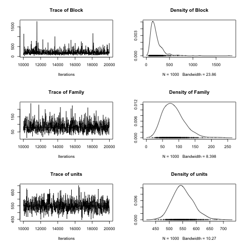
plot(mcmc.list(m4$VCV))
autocorr(m4$VCV)
posterior.mode(m4$VCV)
# Block Family units
#126.66633 72.97771 542.42237
HPDinterval(m4$VCV)
# lower upper
#Block 33.12823 431.0233
#Family 26.34490 146.6648
#units 479.24201 627.7724
The first difference is that we have to specify priors for the coefficients that we would like to estimate (by default fixed effects, the overall intercept for our example, start with a zero mean and very large variance: 106). The phenotypic variance for our response is around 780, which I split into equal parts for Block, Family and Residuals. For each random effect we have provided our prior for the variance (V) and a degree of belief on our prior (n).
In addition to the model equation, name of the data set and prior information we need to specify things like the number of iterations in the chain (nitt), how many we are discarding for the initial burnin period (burnin), and how many values we are keeping (thin, every ten). Besides the pretty plot of the posterior distributions (see previous figure) they can be summarized using the posterior mode and high probability densities.
One of the neat things we can do is to painlessly create functions of variance components and get their posterior mode and credible interval. For example, the heritability (or degree of additive genetic control) can be estimated in this trial with full-sib families using the following formula: \(\hat{h^2} = \frac{2 \sigma_F^2}{\sigma_F^2 + \sigma_B^2 + \sigma_R^2}\)
h2 <- 2 * m4$VCV[, 'Family']/(m4$VCV[, 'Family'] +
          m4$VCV[, 'Block'] + m4$VCV[, 'units'])
plot(h2)

posterior.mode(h2)
#0.1887017

HPDinterval(h2)
#          lower     upper
#var1 0.05951232 0.3414216
#attr(,"Probability")
#[1] 0.95
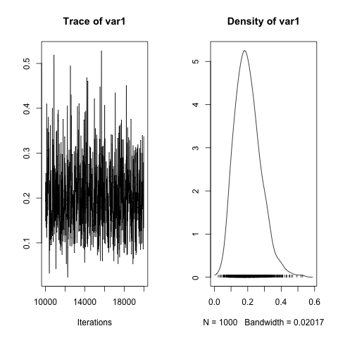
There are some differences on the final results between ASReml-R/lme4 and MCMCglmm; however, the gammas (ratios of variance component/error variance) for the posterior distributions are very similar, and the estimated heritabilities are almost identical (~0.19 vs ~0.21). Overall, MCMCglmm is a very interesting package that covers a lot of ground. It pays to read the reference manual and vignettes, which go into a lot of detail on how to specify different types of models. I will present the MCMCglmm bivariate analyses in another post.
P.S. There are several other ways that we could fit this model in R using a Bayesian approach: it is possible to call WinBugs or JAGS (in Linux and OS X) from R, or we could have used INLA. More on this in future posts.