A few years ago we had this really cool idea: we had to establish a trial to understand wood quality in context. Sort of following the saying “we don’t know who discovered water, but we are sure that it wasn’t a fish” (attributed to Marshall McLuhan). By now you are thinking WTF is this guy talking about? But the idea was simple; let’s put a trial that had the species we wanted to study (Pinus radiata, a gymnosperm) and an angiosperm (Eucalyptus nitens if you wish to know) to provide the contrast, as they are supposed to have vastly different types of wood. From space the trial looked like this:
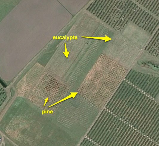
The reason you can clearly see the pines but not the eucalypts is because the latter were dying like crazy over a summer drought (45% mortality in one month). And here we get to the analytical part: we will have a look only at the eucalypts where the response variable can’t get any clearer, trees were either totally dead or alive. The experiment followed a randomized complete block design, with 50 open-pollinated families in 48 blocks. The original idea was to harvest 12 blocks each year but—for obvious reasons—we canned this part of the experiment after the first year.
The following code shows the analysis in asreml-R, lme4 and MCMCglmm:
load('~/Dropbox/euc.Rdata')
library(asreml)
sasreml <- asreml(surv ~ 1, random = ~ Fami + Block,
data = euc,
family = asreml.binomial(link = 'logit'))
summary(sasreml)$varcomp
# gamma component std.error z.ratio
#Fami!Fami.var 0.5704205 0.5704205 0.14348068 3.975591
#Block!Block.var 0.1298339 0.1298339 0.04893254 2.653324
#R!variance 1.0000000 1.0000000 NA NA
# constraint
#Fami!Fami.var Positive
#Block!Block.var Positive
#R!variance Fixed
# Quick look at heritability
varFami <- summary(sasreml)$varcomp[1, 2]
varRep <- summary(sasreml)$varcomp[2, 2]
h2 <- 4*varFami/(varFami + varRep + 3.29)
h2
#[1] 0.5718137
library(lme4)
slme4 <- lmer(surv ~ 1 + (1|Fami) + (1|Block),
data = euc,
family = binomial(link = 'logit'))
summary(slme4)
#Generalized linear mixed model fit by the Laplace approximation
#Formula: surv ~ 1 + (1 | Fami) + (1 | Block)
# Data: euc
# AIC BIC logLik deviance
# 2725 2742 -1360 2719
#Random effects:
# Groups Name Variance Std.Dev.
# Fami (Intercept) 0.60941 0.78065
# Block (Intercept) 0.13796 0.37143
#Number of obs: 2090, groups: Fami, 51; Block, 48
#
#Fixed effects:
# Estimate Std. Error z value Pr(>|z|)
#(Intercept) 0.2970 0.1315 2.259 0.0239 *
# Quick look at heritability
varFami <- VarCorr(slme4)$Fami[1]
varRep <- VarCorr(slme4)$Block[1]
h2 <- 4*varFami/(varFami + varRep + 3.29)
h2
#[1] 0.6037697
# And let's play to be Bayesians!
library(MCMCglmm)
pr <- list(R = list(V = 1, n = 0, fix = 1),
G = list(G1 = list(V = 1, n = 0.002),
G2 = list(V = 1, n = 0.002)))
sb <- MCMCglmm(surv ~ 1,
random = ~ Fami + Block,
family = 'categorical',
data = euc,
prior = pr,
verbose = FALSE,
pr = TRUE,
burnin = 10000,
nitt = 100000,
thin = 10)
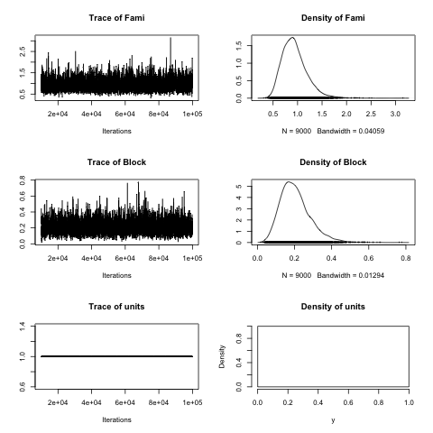
plot(sb$VCV)
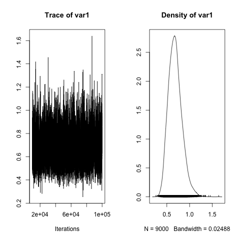
You may be wondering Where does the 3.29 in the heritability formula comes from? Well, that’s the variance of the link function that, in the case of the logit link is pi*pi/3. In the case of MCMCglmm we can estimate the degree of genetic control quite easily, remembering that we have half-siblings (open-pollinated plants):
# Heritability
h2 <- 4*sb$VCV[, 'Fami']/(sb$VCV[, 'Fami'] +
        sb$VCV[, 'Block'] + 3.29 + 1)
posterior.mode(h2)
#     var1
#0.6476185

HPDinterval(h2)
#         lower     upper
#var1 0.4056492 0.9698148
#attr(,"Probability")
#[1] 0.95

plot(h2)
By the way, it is good to remember that we need to back-transform the estimated effects to probabilities, with very simple code:
# Getting mode and credible interval for solutions
inv.logit(posterior.mode(sb$Sol))
inv.logit(HPDinterval(sb$Sol, 0.95))
Even if one of your trials is trashed there is a silver lining: it is possible to have a look at survival.