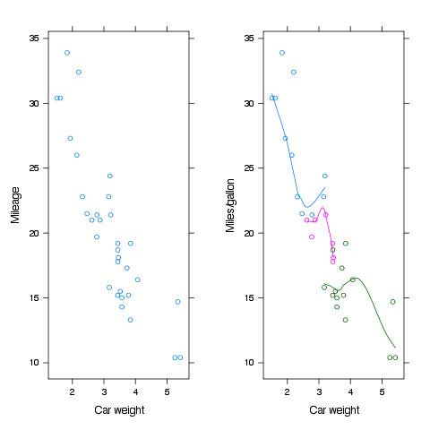
Setting plots side by side
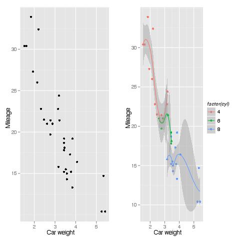
This is simple example code to display side-by-side lattice plots or ggplot2 plots, using the mtcars dataset that comes with any R installation. We will display a scatterplot of miles per US gallon (mpg) on car weight (wt) next to another scatterplot of the same data, but using different colors by number of engine cylinders (cyl, treated as factor) and adding a smooth line (under the type option).
library(lattice)
data(mtcars)

# Create first plot and assign it to variable
p1 <- xyplot(mpg ~ wt, data = mtcars,
             xlab = 'Car weight', ylab = 'Mileage')

# Create second plot and assign it to variable
p2 <- xyplot(mpg ~ wt, group= factor(cyl), data = mtcars,
             xlab = 'Car weight', ylab = 'Miles/gallon',
             type = c('p', 'smooth'))

# print calls print.lattice, which takes a position
# argument.
print(p1, position = c(0, 0, 0.5, 1), more = TRUE)
print(p2, position = c(0.5, 0, 1, 1))

According to the documentation, position is a vector of 4 numbers, typically c(xmin, ymin, xmax, ymax) that give the lower-left and upper-right corners of a rectangle in which the Trellis plot of x is to be positioned. The coordinate system for this rectangle is [0-1] in both the x and y directions. That is, the first print() sets position to occupy the left part of the graph with full height, as well as to avoid refreshing the graph when displaying the new plot (more = TRUE). The second print() uses the right part of the graph with full height.
In the case of ggplot2, the code is not that different:
library(grid)
library(ggplot2)

# Create first plot and assign it to variable
p1 <- qplot(wt, mpg, data = mtcars,
            xlab = 'Car weight', ylab = 'Mileage')

# Create second plot and assign it to variable
p2 <- qplot(wt, mpg, color = factor(cyl), data = mtcars,
            geom = c('point', 'smooth'),
            xlab = 'Car weight', ylab = 'Mileage')

# Define grid layout to locate plots and print each graph
pushViewport(viewport(layout = grid.layout(1, 2)))
print(p1, vp = viewport(layout.pos.row = 1, layout.pos.col = 1))
print(p2, vp = viewport(layout.pos.row = 1, layout.pos.col = 2))

More details on ggplot’s notation can be found here.