Multivariate linear mixed models: livin’ la vida loca
I swear there was a point in writing an introduction to covariance structures: now we can start joining all sort of analyses using very similar notation. In a previous post I described simple (even simplistic) models for a single response variable (or ‘trait’ in quantitative geneticist speak). The R code in three R packages (asreml-R, lme4 and nlme) was quite similar and we were happy-clappy with the consistency of results across packages. The curse of the analyst/statistician/guy who dabbles in analyses is the idea that we can always fit a nicer model and—as both Bob the Builder and Obama like to say—yes, we can.
Let’s assume that we have a single trial where we have assessed our experimental units (trees in my case) for more than one response variable; for example, we measured the trees for acoustic velocity (related to stiffness) and basic density. If you don’t like trees, think of having height and body weight for people, or whatever picks your fancy. Anyway, we have our traditional randomized complete block design with random blocks, random families and that’s it. Rhetorical question: Can we simultaneously run an analysis for all responses?
setwd('~/Dropbox/quantumforest')
library(asreml)
canty <- read.csv('canty_trials.csv', header = TRUE)
summary(canty)

m1 <- asreml(bden ~ 1, random = ~ Block + Family, data = canty)
summary(m1)$varcomp

gamma component std.error   z.ratio constraint
Block!Block.var   0.2980766 162.74383  78.49271  2.073362   Positive
Family!Family.var 0.1516591  82.80282  29.47153  2.809587   Positive
R!variance        1.0000000 545.97983  37.18323 14.683496   Positive


m2 <- asreml(veloc ~ 1, random = ~ Block + Family, data = canty)
summary(m2)$varcomp

gamma   component    std.error   z.ratio constraint
Block!Block.var   0.1255846 0.002186295 0.0011774906  1.856741   Positive
Family!Family.var 0.1290489 0.002246605 0.0008311341  2.703059   Positive
R!variance        1.0000000 0.017408946 0.0012004136 14.502456   Positive
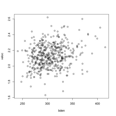
Up to this point we are using the same old code, and remember that we could fit the same model using lme4, so what’s the point of this post? Well, we can now move to fit a multivariate model, where we have two responses at the same time (incidentally, below we have a plot of the two response variables, showing a correlation of ~0.2).

We can first refit the model as a multivariate analysis, assuming block-diagonal covariance matrices. The notation now includes:
- The use of
cbind()to specify the response matrix, - the reserved keyword
trait, which creates a vector to hold the overall mean for each response, at(trait), which asks ASReml-R to fit an effect (e.g. Block) at each trait, by default using a diagonal covariance matrix (σ2 I). We could also usediag(trait)for the same effect,rcov = ~ units:diag(trait)specifies a different diagonal matrix for the residuals (units) of each trait.
m3 <- asreml(cbind(bden, veloc) ~ trait,
             random = ~ at(trait):Block +  at(trait):Family, data = canty,
             rcov = ~ units:diag(trait))

summary(m3)$varcomp
gamma    component    std.error
at(trait, bden):Block!Block.var    1.627438e+02 1.627438e+02 78.492736507
at(trait, veloc):Block!Block.var   2.186295e-03 2.186295e-03  0.001177495
at(trait, bden):Family!Family.var  8.280282e+01 8.280282e+01 29.471507439
at(trait, veloc):Family!Family.var 2.246605e-03 2.246605e-03  0.000831134
R!variance                         1.000000e+00 1.000000e+00           NA
R!trait.bden.var                   5.459799e+02 5.459799e+02 37.183234014
R!trait.veloc.var                  1.740894e-02 1.740894e-02  0.001200414
z.ratio constraint
at(trait, bden):Block!Block.var     2.073362   Positive
at(trait, veloc):Block!Block.var    1.856733   Positive
at(trait, bden):Family!Family.var   2.809589   Positive
at(trait, veloc):Family!Family.var  2.703059   Positive
R!variance                                NA      Fixed
R!trait.bden.var                   14.683496   Positive
R!trait.veloc.var                  14.502455   Positive
Initially, you may not notice that the results are identical, as there is a distracting change to scientific notation for the variance components. A closer inspection shows that we have obtained the same results for both traits, but did we gain anything? Not really, as we took the defaults for covariance components (direct sum of diagonal matrices, which assumes uncorrelated traits); however, we can do better and actually tell ASReml-R to fit the correlation between traits for block and family effects as well as for residuals.
m4 <- asreml(cbind(bden, veloc) ~ trait,
             random = ~ us(trait):Block +  us(trait):Family, data = a,
             rcov = ~ units:us(trait))

summary(m4)$varcomp

gamma    component    std.error
trait:Block!trait.bden:bden    1.628812e+02 1.628812e+02 7.854123e+01
trait:Block!trait.veloc:bden   1.960789e-01 1.960789e-01 2.273473e-01
trait:Block!trait.veloc:veloc  2.185595e-03 2.185595e-03 1.205128e-03
trait:Family!trait.bden:bden   8.248391e+01 8.248391e+01 2.932427e+01
trait:Family!trait.veloc:bden  1.594152e-01 1.594152e-01 1.138992e-01
trait:Family!trait.veloc:veloc 2.264225e-03 2.264225e-03 8.188618e-04
R!variance                     1.000000e+00 1.000000e+00           NA
R!trait.bden:bden              5.460010e+02 5.460010e+02 3.712833e+01
R!trait.veloc:bden             6.028132e-01 6.028132e-01 1.387624e-01
R!trait.veloc:veloc            1.710482e-02 1.710482e-02 9.820673e-04
z.ratio constraint
trait:Block!trait.bden:bden     2.0738303   Positive
trait:Block!trait.veloc:bden    0.8624639   Positive
trait:Block!trait.veloc:veloc   1.8135789   Positive
trait:Family!trait.bden:bden    2.8128203   Positive
trait:Family!trait.veloc:bden   1.3996166   Positive
trait:Family!trait.veloc:veloc  2.7650886   Positive
R!variance                             NA      Fixed
R!trait.bden:bden              14.7057812   Positive
R!trait.veloc:bden              4.3442117   Positive
R!trait.veloc:veloc            17.4171524   Positive
Moving from model 3 to model 4 we are adding three covariance components (one for each family, block and residuals) and improving log-likelihood by 8.5. A quick look at the output from m4 would indicate that most of that gain is coming from allowing for the covariance of residuals for the two traits, as the covariances for family and, particularly, block are more modest:
summary(m3)$loglik
[1] -1133.312

summary(m4)$loglik
[1] -1124.781
An alternative parameterization for model 4 would be to use a correlation matrix with heterogeneous variances (corgh(trait) instead of us(trait)), which would model the correlation and the variances instead of the covariance and the variances. This approach seems to be more numerically stable sometimes.
As an aside, we can estimate the between traits correlation for Blocks (probably not that interesting) and the one for Family (much more interesting, as it is an estimate of the genetic correlation between traits: 1.594152e-01 / sqrt(8.248391e01 * 2.264225e-03) = 0.37).