Evolving notes, images and sounds by Luis Apiolaza

Coming out of the (Bayesian) closet: multivariate version

This week I’m facing my—and many other lecturers’—least favorite part of teaching: grading exams. In a supreme act of procrastination I will continue the previous post, and the antepenultimate one, showing the code for a bivariate analysis of a randomized complete block design.

Just to recap, the results from the REML multivariate analysis (that used ASReml-R) was the following:

library(asreml)

m4 <- asreml(cbind(bden, veloc) ~ trait,
             random = ~ us(trait):Block +  us(trait):Family, data = a,
             rcov = ~ units:us(trait))

summary(m4)$varcomp

#                                      gamma    component    std.error
#trait:Block!trait.bden:bden    1.628812e+02 1.628812e+02 7.854123e+01
#trait:Block!trait.veloc:bden   1.960789e-01 1.960789e-01 2.273473e-01
#trait:Block!trait.veloc:veloc  2.185595e-03 2.185595e-03 1.205128e-03
#trait:Family!trait.bden:bden   8.248391e+01 8.248391e+01 2.932427e+01
#trait:Family!trait.veloc:bden  1.594152e-01 1.594152e-01 1.138992e-01
#trait:Family!trait.veloc:veloc 2.264225e-03 2.264225e-03 8.188618e-04
#R!variance                     1.000000e+00 1.000000e+00           NA
#R!trait.bden:bden              5.460010e+02 5.460010e+02 3.712833e+01
#R!trait.veloc:bden             6.028132e-01 6.028132e-01 1.387624e-01
#R!trait.veloc:veloc            1.710482e-02 1.710482e-02 9.820673e-04
#                                  z.ratio constraint
#trait:Block!trait.bden:bden     2.0738303   Positive
#trait:Block!trait.veloc:bden    0.8624639   Positive
#trait:Block!trait.veloc:veloc   1.8135789   Positive
#trait:Family!trait.bden:bden    2.8128203   Positive
#trait:Family!trait.veloc:bden   1.3996166   Positive
#trait:Family!trait.veloc:veloc  2.7650886   Positive
#R!variance                             NA      Fixed
#R!trait.bden:bden              14.7057812   Positive
#R!trait.veloc:bden              4.3442117   Positive
#R!trait.veloc:veloc            17.4171524   Positive

The corresponding MCMCglmm code is not that different from ASReml-R, after which it is modeled anyway. Following the recommendations of the MCMCglmm Course Notes (included with the package), the priors have been expanded to diagonal matrices with degree of belief equal to the number of traits. The general intercept is dropped (-1) so the trait keyword represents trait means. We are fitting unstructured (us(trait)) covariance matrices for both Block and Family, as well as an unstructured covariance matrix for the residuals. Finally, both traits follow a gaussian distribution:

library(MCMCglmm)
bp <- list(R = list(V = diag(c(0.007, 260)), n = 2),
           G = list(G1 = list(V = diag(c(0.007, 260)), n = 2),
           G2 = list(V = diag(c(0.007, 260)), n = 2)))

bmod <- MCMCglmm(cbind(veloc, bden) ~ trait - 1,
                 random = ~ us(trait):Block + us(trait):Family,
                 rcov = ~ us(trait):units,
                 family = c('gaussian', 'gaussian'),
                 data = a,
                 prior = bp,
                 verbose = FALSE,
                 pr = TRUE,
                 burnin = 10000,
                 nitt = 20000,
                 thin = 10)

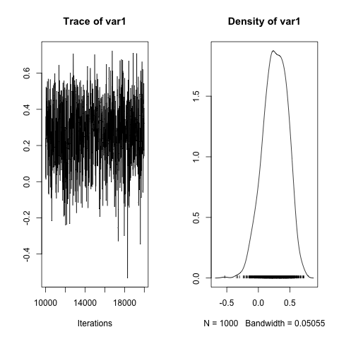
Further manipulation of the posterior distributions requires having an idea of the names used to store the results. Following that, we can build an estimate of the genetic correlation between the traits (Family covariance between traits divided by the square root of the product of the Family variances). Incidentally, it wouldn't be a bad idea to run a much longer chain for this model, so the plot of the posterior for the correlation looks better, but I'm short of time:

dimnames(bmod$VCV)

rg <- bmod$VCV[,'veloc:bden.Family']/sqrt(bmod$VCV[,'veloc:veloc.Family'] *
      bmod$VCV[,'bden:bden.Family'])

plot(rg)

posterior.mode(rg)
#     var1
#0.2221953


HPDinterval(rg, prob = 0.95)
#         lower     upper
#var1 -0.132996 0.5764006
#attr(,"Probability")
#[1] 0.95
And that's it! Time to congratulate Jarrod Hadfield for developing this package.

7 Comments

  1. Rafael Maia

    this is fascinating stuff, thanks for putting up a worked example! I have lots of questions, heh, but I'll start with the main one (and one I guess many people interested in this may have): say you were putting together a mixed model in which you were interested in the effect of a predictor variable as a fixed effect (say, for your example, tree height or root density). How would the coefficient of that effect come out, and how would you interpret it? Would it be a matrix describing the effect on the multivariate normal mean, or a single coefficient that relates in some way to it?

    • Luis

      Caro Rafael,

      It is interesting that you ask about the fixed effects, which I often don't care about except to account for population mean differences in genetic evaluation. I think that we would present the model to something like this: cbind(veloc, bden) ~ trait – 1 + trait:FixedEff, random = ~…
      which would separately fit FixedEff for each trait and store the samples of the posterior under Sol (for solutions). Thus, if we run something like posterior.mode(bmod$Sol) we would get a vector of posterior modes for each of the terms of the model, first the fixed effects (trait 1 mode, trait2 mode, levels of FixedEff) and then random effects (Block and Family levels). We can also get their credible intervals using HPDinterval(bmod$Sol).

      I'm not sure if I am answering your question, but we can keep on chatting.

  2. Rafael Maia

    Thanks for the detailed explanation! So in a sense, it wouldn't be that different to conducting separate univariate analyses (with the exception of the random effect partitioning) for the two response variables – i.e. it doesn't explore the covariance properties of them in estimating the fixed effects?

    • Luis

      My speculation: I think the key part is that we are simultaneously estimating both fixed and random effects, so any flow of information from one trait to the other (via covariances of random effects) will have an impact on the estimation of fixed effects. I'm not totally sure how it works in a Bayesian setting, but I'll be developing some small calculations soon to show the effect using a toy example.

  3. Torvon

    Hey, wonderful practical example! And being a blog person myself, I … revere your font type. It’s fantastic!

    To the issue at hand: I don’t quite understand the parameterization of the prior(s). I didn’t in the coursenotes, and I don’t understand in your example. Would you be willing to explain this a bit more?

    library(MCMCglmm)
    bp = list(R = list(V = diag(c(0.007, 260)), n = 2),
    G = list(G1 = list(V = diag(c(0.007, 260)), n = 2),
    G2 = list(V = diag(c(0.007, 260)), n = 2)))

    Thank you
    T

    • Luis

      Hi Torvon,

      The priors are specified in nested lists. At the top level we have one element for R and one for G; the one for G happens to be a list too, with one element for each random factor.

      For each random factor we have the starting values and an indication of strength of believe. For the bivariate case, the starting values are a matrix, assuming a variance for each trait and zero covariance, which is why they can be started with a diagonal matrix. Somewhere in the manual there is a comment that n should be the number of traits in the analyses.

      So we have:
      * Prior for R
      * Prior for G, which involves:
      ** Prior for G1 (first random effect in the model).
      ** Prior for G2 (second random effect in the model).
      ** etc.

      For each prior we have:
      * Matrix of values.
      * Indication of strength.

      With enough data, your priors will just wash out.

      • Torvon

        Thank you, that was very helpful. Unfortunately, I still don’t seem to get things working. My ordinal, multivariate model with separate regressions from x1 and x2 on each response, correlated subject effects and correlated observation effects is this:

        m1 <- MCMCglmm (cbind (y1,y2) ~ -1 + trait + trait:x1 + trait:x2, random=~us(trait):UserID, rcov=~cor(trait):units, data=data, family=c("ordinal","ordinal"), verbose=FALSE, prior=prior)

        1) prior=list(R=list(V=1, nu=0.002),G=list(V=1, nu=0.002))
        and
        2) prior=list(R=list(V=1, nu=0.002),G=list(G1=list(V=1, nu=0.002)))
        do not work, neither G lists with two ore three Gs.
        ("prior$G has the wrong number of structures").

        What am I doing wrong? I don't quite understand. Thanks a bunch!
        — T

© 2024 Palimpsest

Theme by Anders NorenUp ↑