Analyzing a simple experiment with heterogeneous variances using asreml, MCMCglmm and SAS
I was working with a small experiment which includes families from two Eucalyptus species and thought it would be nice to code a first analysis using alternative approaches. The experiment is a randomized complete block design, with species as fixed effect and family and block as a random effects, while the response variable is growth strain (in
$$\mu \epsilon$$).
When looking at the trees one can see that the residual variances will be very different. In addition, the trees were growing in plastic bags laid out in rows (the blocks) and columns. Given that trees were growing in bags siting on flat terrain, most likely the row effects are zero.
Below is the code for a first go in R (using both MCMCglmm and ASReml-R) and SAS. I had stopped using SAS for several years, mostly because I was running a mac for which there is no version. However, a few weeks ago I started accessing it via their OnDemand for Academics program via a web browser.
The R code using REML looks like:
# Options
options(stringsAsFactors = FALSE)
setwd('~/Dropbox/research/2013/growth-stress')

# Packages
library(ggplot2)
library(asreml)
library(MCMCglmm)


# Reading data, renaming, factors, etc
gs <- read.csv('eucalyptus-growth-stress.csv')
summary(gs)

# Both argophloia and bosistoana
gsboth <- subset(gs, !is.na(strain))
gsboth <- within(gsboth, {
  species <- factor(species)
  row <- factor(row)
  column <- factor(column)
  fam <- factor(fam)
})

ma <- asreml(strain ~ species, random = ~ fam + row,
             rcov = ~ at(species):units,
             data = gsboth)

summary(ma)$varcomp

#                                   gamma  component std.error   z.ratio constraint
#fam!fam.var                    27809.414  27809.414 10502.036 2.6480022   Positive
#row!row.var                     2337.164   2337.164  3116.357 0.7499666   Positive
#species_E.argopholia!variance 111940.458 111940.458 26609.673 4.2067580   Positive
#species_E.bosistoana!variance  63035.256  63035.256  7226.768 8.7224681   Positive
While using MCMC we get estimates in the ballpark by using:
# Priors
bothpr <- list(R = list(V = diag(c(50000, 50000)), nu = 3),
               G = list(G1 = list(V = 20000, nu = 0.002),
               G2 = list(V = 20000, nu = 0.002),
               G3 = list(V = 20000, nu = 0.002)))

# MCMC
m2 <- MCMCglmm(strain ~ species, random = ~ fam + row + column,
   rcov = ~ idh(species):units,
  data = gsboth,
  prior = bothpr,
  pr = TRUE,
  family = 'gaussian',
  burnin = 10000,
  nitt = 40000,
  thin = 20,
  saveX = TRUE,
  saveZ = TRUE,
  verbose = FALSE)

summary(m2)

# Iterations = 10001:39981
# Thinning interval  = 20
# Sample size  = 1500
#
# DIC: 3332.578
#
# G-structure:  ~fam
#
# post.mean l-95% CI u-95% CI eff.samp
# fam     30315    12211    55136     1500
#
# ~row
#
# post.mean l-95% CI u-95% CI eff.samp
# row      1449    5.928     6274    589.5
#
# R-structure:  ~idh(species):units
#
# post.mean l-95% CI u-95% CI eff.samp
# E.argopholia.units    112017    71152   168080     1500
# E.bosistoana.units     65006    52676    80049     1500
#
# Location effects: strain ~ species
#
# post.mean l-95% CI u-95% CI eff.samp  pMCMC
# (Intercept)            502.21   319.45   690.68     1500 <7e-04 ***
# speciesE.bosistoana   -235.95  -449.07   -37.19     1361  0.036 *
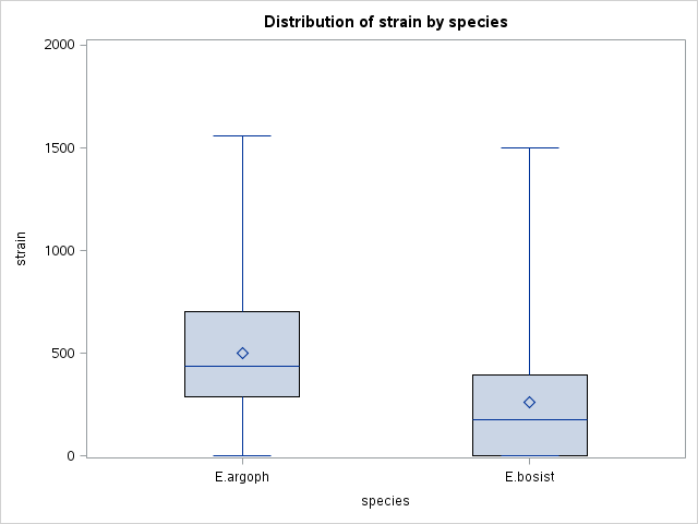
The SAS code is not that disimilar, except for the clear demarcation between data processing (data step, for reading files, data transformations, etc) and specific procs (procedures), in this case to summarize data, produce a boxplot and fit a mixed model.
* termstr=CRLF accounts for the windows-like line endings of the data set;
data gs;
  infile "/home/luis/Projects/euc-strain/growthstresses.csv"
  dsd termstr=CRLF firstobs=2;
  input row column species $ family $ strain;
  if strain ^= .;
run;

proc summary data = gs print;
  class species;
  var strain;
run;

proc boxplot data = gs;
  plot strain*species;
run;

proc mixed data = gs;
  class row species family;
  model strain = species;
  random row family;
  repeated species / group=species;
run;

/*
Covariance Parameter Estimates
Cov Parm     Group                    Estimate
row                                  2336.80
family                                  27808
species     species E.argoph     111844
species     species E.bosist     63036
*/

I like working with multiple languages and I realized that, in fact, I missed SAS a bit. It was like meeting an old friend; at the beginning felt strange but we were quickly chatting away after a few minutes.