Cute Gibbs sampling for rounded observations
I was attending a course of Bayesian Statistics where this problem showed up:
There is a number of individuals, say 12, who take a pass/fail test 15 times. For each individual we have recorded the number of passes, which can go from 0 to 15. Because of confidentiality issues, we are presented with rounded-to-the-closest-multiple-of-3 data \(\mathbf{R}\). We are interested on estimating \(\theta\) of the Binomial distribution behind the data.
Rounding is probabilistic, with probability 2/3 if you are one count away from a multiple of 3 and probability 1/3 if the count is you are two counts away. Multiples of 3 are not rounded.
We can use Gibbs sampling to alternate between sampling the posterior for the unrounded \(\mathbf{Y}\) and \(\theta\). In the case of \(\mathbf{Y}\) I used:
# Possible values that were rounded to R
possible <- function(rounded) {
if(rounded == 0) {
  options <- c(0, 1, 2)
} else {
  options <- c(rounded - 2, rounded - 1, rounded,
               rounded + 1, rounded + 2)
}
  return(options)
}

# Probability mass function of numbers rounding to R
# given theta
prior_y <- function(options, theta) {
  p <- dbinom(options, 15, prob = theta)
  return(p)
}

# Likelihood of rounding
like_round3 <- function(options) {
  if(length(options) == 3) {
    like <- c(1, 2/3, 1/3) }
  else {
    like <- c(1/3, 2/3, 1, 2/3, 1/3)
  }
  return(like)
}

# Estimating posterior mass function and drawing a
# random value of it
posterior_sample_y <- function(R, theta) {
  po <- possible(R)
  pr <- prior_y(po, theta)
  li <- like_round3(po)
  post <- li*pr/sum(li*pr)
  samp <- sample(po, 1, prob = post)
  return(samp)
}
While for \(\theta\) we are assuming a vague \(Beta(\alpha, \beta)\), with \(\alpha\) and \(\beta\) equal to 1, as prior density function for \(\theta\), so the posterior density is a
$$Beta(\alpha + \sum Y_i, \beta + 12*15 - \sum Y_i)$$.
## Function to sample from the posterior Pr(theta | Y, R)
posterior_sample_theta <- function(alpha, beta, Y) {
  theta <- rbeta(1, alpha + sum(Y), beta + 12*15 - sum(Y))
return(theta)
}
I then implemented the sampler as:
## Data
R <- c(0, 0, 3, 9, 3, 0, 6, 3, 0, 6, 0, 3)
nsim <- 10000
burnin <- 1000
alpha <- 1
beta <- 1
store <- matrix(0, nrow = nsim, ncol = length(R) + 1)
starting.values <- c(R, 0.1)
## Sampling
store[1,] <- starting.values
for(draw in 2:nsim){
  current <- store[draw - 1,]
  for(obs in 1:length(R)) {
    y <- posterior_sample_y(R[obs],
                            current[length(R) + 1])
    # Jump or not still missing
    current[obs] <- y
  }
  theta <- posterior_sample_theta(alpha, beta,
                                  current[1:length(R)])
  # Jump or not still missing
  current[length(R) + 1] <- theta
  store[draw,] <- current
}
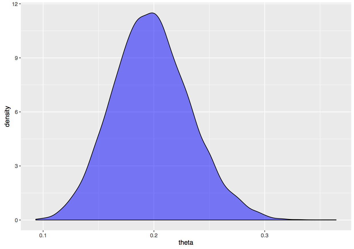
And plotted the results as:
plot((burnin+1):nsim, store[(burnin+1):nsim,13],
     type = 'l')

library(ggplot2)
ggplot(data.frame(theta = store[(burnin+1):nsim,13]),
  aes(x = theta)) +
  geom_density(fill = 'blue', alpha = 0.5)
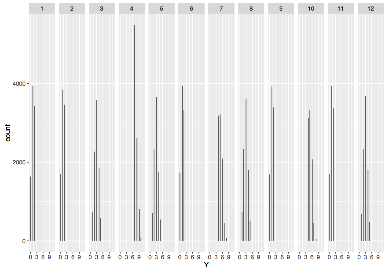
multiple_plot <- data.frame(Y = matrix(store[(burnin+1):nsim, 1:12],
                            nrow = (nsim - burnin)*12,
                            ncol = 1))
multiple_plot$obs <- factor(rep(1:12,
                            each = (nsim - burnin)))
ggplot(multiple_plot, aes(x = Y)) +
  geom_histogram() + facet_grid(~ obs)
I thought it was a nice, cute example of simultaneously estimating a latent variable and, based on that, estimating the parameter behind it.