Turtles all the way down
One of the main uses for R is for exploration and learning. Let’s say that I wanted to learn simple linear regression (the bread and butter of statistics) and see how the formulas work. I could simulate a simple example and fit the regression with R:
library(arm) # For display()
# Simulate 5 observations
set.seed(50)
x <- 1:5
y <- 2 + 3*x + rnorm(5, mean = 0, sd = 3)
# Fit regression
reg <- lm(y ~ x, dat)
display(reg)
# lm(formula = y ~ x, data = dat)
# coef.est coef.se
# (Intercept) 3.99 3.05
# x 2.04 0.92
# ---
# n = 5, k = 2
# residual sd = 2.91, R-Squared = 0.62
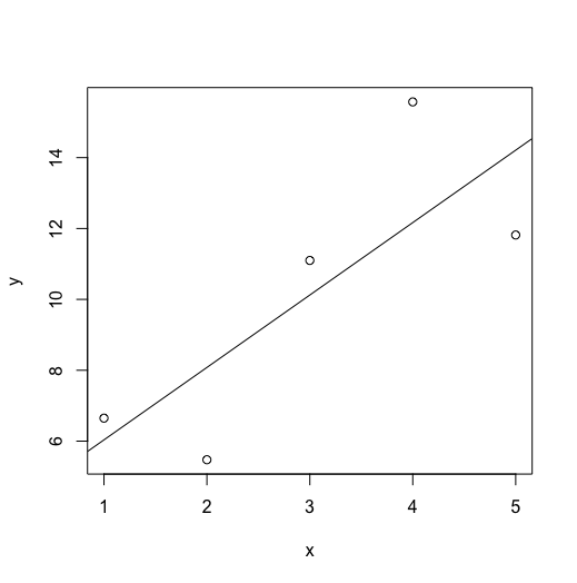
# Plot it
plot(y ~ x)
abline(coef(reg))
The formulas for the intercept (
$$b_0$$) and the slope (
$$b_1$$) are pretty simple, and I have been told that there is a generic expression that instead uses matrices.
$$b_1 = \frac{\sum{x y} - n \bar{x} \bar{y}}{\sum{x x} - n \bar{x}^2}$$
How do the contents of the matrices and the simple formulates relate to each other?
# Formulas for slope and intercept
b1 <- (sum(x*y) - length(x)*mean(x)*mean(y))/(sum(x*x) - length(x)*mean(x)^2)
b0 <- mean(y) - b1*mean(x)
Funnily enough, looking at the matrices we can see similar sums of squares and crossproducts as in the formulas.
X <- model.matrix(reg)

#   (Intercept) x
# 1           1 1
# 2           1 2
# 3           1 3
# 4           1 4
# 5           1 5
# attr(,"assign")
# [1] 0 1

t(X) %*% X
#             (Intercept)  x
# (Intercept)           5 15
# x                    15 55

# So X`X contains bits and pieces of the previous formulas
length(x)
# [1] 5

sum(x)
# [1] 15

sum(x*x)
# [1] 55

# And so does X`y
t(X) %*% y
#                  [,1]
# (Intercept)  50.61283
# x           172.27210

sum(y)
# [1] 50.61283

sum(x*y)
# [1] 172.2721

# So if we combine the whole lot and remember that
# solves calculates the inverse
solve(t(X) %*% X) %*% t(X) %*% y
#                 [,1]
# (Intercept) 3.992481
# x           2.043362
But I have been told that R (as most statistical software) doesn’t use the inverse of the matrix for estimating the coefficients. So how does it work?
If I type lm R will print the code of the lm() function. A quick look will reveal that there is a lot of code reading the arguments and checking that everything is OK before proceeding. However, the function then calls something else: lm.fit(). With some trepidation I type lm.fit, which again performs more checks and then calls something with a different notation:
z <- .Call(C_Cdqrls, x, y, tol, FALSE)
This denotes a call to a C language function, which after some searching in Google we find in a readable form in the lm.c file. Another quick look brings more checking and a call to Fortran code:
F77_CALL(dqrls)(REAL(qr), &n, &p, REAL(y), &ny, &rtol,
		    REAL(coefficients), REAL(residuals), REAL(effects),
		    &rank, INTEGER(pivot), REAL(qraux), work);
which is a highly tuned routine for QR decomposition in a linear algebra library. By now we know that the general matrix expression produces the same as our initial formula, and that the R lm() function does not use a matrix inverse but QR decomposition to solve the system of equations.
One of the beauties of R is that brought the power of statistical computing to the masses, by not only letting you fit models but also having a peek at how things are implemented. As a user, I don’t need to know that there is a chain of function calls initiated by my bread-and-butter linear regression. But it is comforting to the nerdy me, that I can have a quick look at that.
All this for free, which sounds like a very good deal to me.