Large applications of linear mixed models
In a previous post I summarily described our options for (generalized to varying degrees) linear mixed models from a frequentist point of view: nlme, lme4 and ASReml-R†, followed by a quick example for a split-plot experiment.
But who is really happy with a toy example? We can show a slightly more complicated example assuming that we have a simple situation in breeding: a number of half-sib trials (so we have progeny that share one parent in common), each of them established following a randomized complete block design, analyzed using a ‘family model’. That is, the response variable (dbh: tree stem diameter assessed at breast height—1.3m from ground level) can be expressed as a function of an overall mean, fixed site effects, random block effects (within each site), random family effects and a random site-family interaction. The latter provides an indication of genotype by environment interaction.
setwd('~/Dropbox/quantumforest')

trees <- read.table('treedbh.txt', header=TRUE)

# Removing all full-siblings and dropping Trial levels
# that are not used anymore
trees <- subset(trees, Father == 0)
trees$Trial <- trees$Trial[drop = TRUE]

# Which let me with 189,976 trees in 31 trials
xtabs(~Trial, data = trees)

# First run the analysis with lme4
library(lme4)
m1 <- lmer(dbh ~ Trial + (1|Trial:Block) + (1|Mother) +
           (1|Trial:Mother), data = trees)


# Now run the analysis with ASReml-R
library(asreml)
m2 <- asreml(dbh ~ Trial, random = ~Trial:Block + Mother +
             Trial:Mother, data = trees)
First I should make clear that this model has several drawbacks:
- It assumes that we have homogeneous variances for all trials, as well as identical correlation between trials. That is, that we are assuming compound symmetry, which is very rarely the case in multi-environment progeny trials.
- It also assumes that all families are unrelated to each other, which in this case I know it is not true, as a quick look at the pedigree will show that several mothers are related.
- We assume only one type of families (half-sibs), which is true just because I got rid of all the full-sib families and clonal material, to keep things simple in this example.
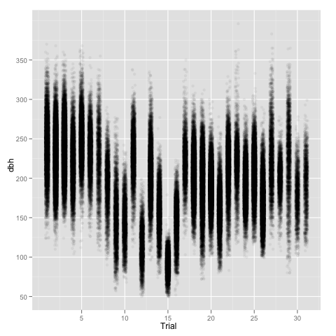
Just to make the point, a quick look at the data using ggplot2—with some jittering and alpha transparency to better display a large number of points—shows differences in both mean and variance among sites.
library(ggplot2)
ggplot(aes(x=jitter(as.numeric(Trial)), y=dbh), data = trees) +
  geom_point(colour=alpha('black', 0.05)) +
  scale_x_continuous('Trial')

Anyway, let’s keep on going with this simplistic model. In my computer, a two year old iMac, ASReml-R takes roughly 9 seconds, while lme4 takes around 65 seconds, obtaining similar results.
# First lme4 (and rounding off the variances)
summary(m1)

Random effects:
Groups       Name        Variance Std.Dev.
Trial:Mother (Intercept)  26.457   5.1436
Mother       (Intercept)  32.817   5.7286
Trial:Block  (Intercept)  77.390   8.7972
Residual                 892.391  29.8729


# And now ASReml-R
# Round off part of the variance components table
round(summary(m2)$varcomp[,1:4], 3)
gamma component std.error z.ratio
Trial:Block!Trial.var  0.087    77.399     4.598  16.832
Mother!Mother.var      0.037    32.819     1.641  20.002
Trial:Mother!Trial.var 0.030    26.459     1.241  21.328
R!variance             1.000   892.389     2.958 301.672
The residual matrix of this model is a, fairly large, diagonal matrix (residual variance times an identity matrix). At this point we can relax this assumption, adding a bit more complexity to the model so we can highlight some syntax. Residuals in one trial should have nothing to do with residuals in another trial, which could be hundreds of kilometers away. I will then allow for a new matrix of residuals, which is the direct sum of trial-specific diagonal matrices. In ASReml-R we can do so by specifying a diagonal matrix at each trial with rcov = ~ at(Trial):units:
m2b <-  asreml(dbh ~ Trial, random = ~Trial:Block + Mother +
               Trial:Mother, data = trees,
               rcov = ~ at(Trial):units)

# Again, extracting and rounding variance components
round(summary(m2b)$varcomp[,1:4], 3)
gamma component std.error z.ratio
Trial:Block!Trial.var    77.650    77.650     4.602  16.874
Mother!Mother.var        30.241    30.241     1.512  20.006
Trial:Mother!Trial.var   22.435    22.435     1.118  20.065
Trial_1!variance       1176.893  1176.893    18.798  62.606
Trial_2!variance       1093.409  1093.409    13.946  78.403
Trial_3!variance        983.924   983.924    12.061  81.581
...
Trial_29!variance      2104.867  2104.867    55.821  37.708
Trial_30!variance       520.932   520.932    16.372  31.819
Trial_31!variance       936.785   936.785    31.211  30.015
There is a big improvement of log-Likelihood from m2 (-744452.1) to m2b (-738011.6) for 30 additional variances. At this stage, we can also start thinking of heterogeneous variances for blocks, with a small change to the code:
m2c <-  asreml(dbh ~ Trial,
               random = ~at(Trial):Block + Mother +
               Trial:Mother, data = wood,
               rcov = ~ at(Trial):units)
round(summary(m2c)$varcomp[,1:4], 3)

# Which adds another 30 variances (one for each Trial)
gamma component std.error z.ratio
at(Trial, 1):Block!Block.var     2.473     2.473     2.268   1.091
at(Trial, 2):Block!Block.var    95.911    95.911    68.124   1.408
at(Trial, 3):Block!Block.var     1.147     1.147     1.064   1.079
...
Mother!Mother.var               30.243    30.243     1.512  20.008
Trial:Mother!Trial.var          22.428    22.428     1.118  20.062
Trial_1!variance              1176.891  1176.891    18.798  62.607
Trial_2!variance              1093.415  1093.415    13.946  78.403
Trial_3!variance               983.926   983.926    12.061  81.581
...
At this point we could do extra modeling at the site level by including any other experimental design features, allowing for spatially correlated residuals, etc. I will cover some of these issues in future posts, as this one is getting a bit too long. However, we could gain even more by expressing the problem in a multivariate fashion, where the performance of Mothers in each trial would be considered a different trait. This would push us towards some large problems, which require modeling covariance structures so we have a change of achieving convergence during our lifetime.
Disclaimer: I am emphasizing the use of ASReml-R because 1.- I am most familiar with it than with nlme or lme4 (although I tend to use nlme for small projects), and 2.- There are plenty of examples for the other packages but not many for ASReml in the R world. I know some of the people involved in the development of ASReml-R but otherwise I have no commercial links with VSN (the guys that market ASReml and Genstat).
† There are other packages that I have not had the chance to investigate yet, like hglm.