Spatial correlation in designed experiments

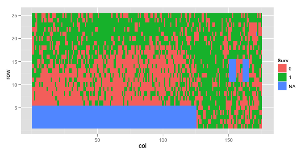
Last Wednesday I had a meeting with the folks of the New Zealand Drylands Forest Initiative in Blenheim. In addition to sitting in a conference room and having nice sandwiches we went to visit one of our progeny trials at Cravens. Plantation forestry trials are usually laid out following a rectangular lattice defined by rows and columns. The trial follows an incomplete block design with 148 blocks and is testing 60 Eucalyptus bosistoana families. A quick look at survival shows an interesting trend: the bottom of the trial was much more affected by frost than the top.

setwd('~/Dropbox/quantumforest')
library(ggplot2) # for qplot
library(asreml)

load('cravens.Rdata')

qplot(col, row, fill = Surv, geom='tile', data = cravens)

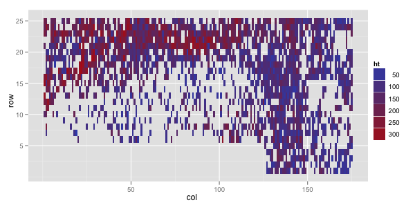
We have the trial assessed for tree height (ht) at 2 years of age, where a plot also shows some spatial trends, with better growth on the top-left corner; this is the trait that I will analyze here.

Tree height can be expressed as a function of an overall constant, random block effects, random family effects and a normally distributed residual (this is our base model, m1). I will then take into account the position of the trees (expressed as rows and columns within the trial) to fit spatially correlated residuals (m2)—using separable rows and columns processes—to finally add a spatially independent residual to the mix (m3).

# Base model (non-spatial)
m1 <- asreml(ht ~ 1, random = ~ Block + Family, data = cravens)
summary(m1)$loglik
[1] -8834.071

summary(m1)$varcomp

gamma component std.error   z.ratio constraint
Block!Block.var   0.52606739 1227.4058 168.84681  7.269345   Positive
Family!Family.var 0.06257139  145.9898  42.20675  3.458921   Positive
R!variance        1.00000000 2333.1722  78.32733 29.787459   Positive

m1 represents a traditional family model with only the overall constant as the only fixed effect and a diagonal residual matrix (identity times the residual variance). In m2 I am modeling the R matrix as the Kronecker product of two separable autoregressive processes (one in rows and one in columns) times a spatial residual.

# Spatial model (without non-spatial residual)
m2 <- asreml(ht ~ 1, random = ~ Block + Family,
             rcov = ~ ar1(row):ar1(col),
             data = cravens[order(cravens$row, cravens$col),])
summary(m2)$loglik
[1] -8782.112

summary(m2)$varcomp

gamma    component    std.error   z.ratio
Block!Block.var   0.42232303 1025.9588216 157.00799442  6.534437
Family!Family.var 0.05848639  142.0822874  40.20346956  3.534080
R!variance        1.00000000 2429.3224308  88.83064209 27.347798
R!row.cor         0.09915320    0.0991532   0.02981808  3.325271
R!col.cor         0.28044024    0.2804402   0.02605972 10.761445

constraint
Block!Block.var         Positive
Family!Family.var       Positive
R!variance              Positive
R!row.cor          Unconstrained
R!col.cor          Unconstrained

Adding two parameters to the model results in improving the log-likelihood from -8834.071 to -8782.112, a difference of 51.959, but with what appears to be a low correlation in both directions. In m3 I am adding an spatially independent residual (using the keyword units), improving log-likelihood from -8782.112 to -8660.411: not too shabby.

m3 <- asreml(ht ~ 1, random = ~ Block + Family + units,
             rcov = ~ ar1(row):ar1(col),
             data = cravens[order(cravens$row, cravens$col),])
summary(m3)$loglik
[1] -8660.411

summary(m3)$varcomp

gamma    component    std.error    z.ratio
Block!Block.var   3.069864e-07 4.155431e-04 6.676718e-05   6.223763
Family!Family.var 1.205382e-01 1.631630e+02 4.327885e+01   3.770040
units!units.var   1.354166e+00 1.833027e+03 7.085134e+01  25.871456
R!variance        1.000000e+00 1.353621e+03 2.174923e+02   6.223763
R!row.cor         7.814065e-01 7.814065e-01 4.355976e-02  17.938724
R!col.cor         9.529984e-01 9.529984e-01 9.100529e-03 104.719017
constraint
Block!Block.var        Boundary
Family!Family.var      Positive
units!units.var        Positive
R!variance             Positive
R!row.cor         Unconstrained
R!col.cor         Unconstrained

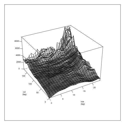
Allowing for the independent residual (in addition to the spatial one) has permitted higher autocorrelations (particularly in columns), while the Block variance has gone very close to zero. Most of the Block variation is being captured now through the residual matrix (in the rows and columns autoregressive correlations), but we are going to keep it in the model, as it represents a restriction to the randomization process. In addition to log-likelihood (or AIC) we can get graphical descriptions of the fit by plotting the empirical semi-variogram as in plot(variogram(m3)):