Split-plot 1: How does a linear mixed model look like?
I like statistics and I struggle with statistics. Often times I get frustrated when I don’t understand and I really struggled to make sense of Krushke’s Bayesian analysis of a split-plot, particularly because ‘it didn’t look like’ a split-plot to me.
Additionally, I have made a few posts discussing linear mixed models using several different packages to fit them. At no point I have shown what are the calculations behind the scenes. So, I decided to combine my frustration and an explanation to myself in a couple of posts. This is number one and the follow up is Split-plot 2: let’s throw in some spatial effects.

How do linear mixed models look like #
Linear mixed models, models that combine so-called fixed and random effects, are often represented using matrix notation as
$$\mathbf{y} = \mathbf{X b} + \mathbf{Z a} + \mathbf{e}$$where $\mathbf{y}$ represents the response variable vector, $\mathbf{X}$ and $\mathbf{Z}$ are incidence matrices relating the response to the fixed $\mathbf{b}$ e.g. overall mean, treatment effects, etc) and random (\mathbf{a}$$), e.g. family effects, additive genetic effects and a host of experimental design effects like blocks, rows, columns, plots, etc), and last the random residuals ($\mathbf{e}$).
The previous model equation still requires some assumptions about the distribution of the random effects. A very common set of assumptions is to say that the residuals are iid (identical and independently distributed) normal (so $\mathbf{R} = \sigma^2_e \mathbf{I}$) and that the random effects are independent of each other, so $\mathbf{G} = \mathbf{B} \bigoplus \mathbf{M}$ is a direct sum of the variance of blocks $\mathbf{B} = \sigma^2_B \mathbf{I}$ and main plots ($\mathbf{M} = \sigma^2_M \mathbf{I}$).
An interesting feature of this matrix formulation is that we can express all sort of models by choosing different assumptions for our covariance matrices (using different covariance structures). Do you have longitudinal data (units assessed repeated times)? Is there spatial correlation? Account for this in the
$$\mathbf{R}$$matrix. Random effects are correlated (e.g. maternal and additive genetic effects in genetics)? Account for this in the
$$\mathbf{G}$$matrix. Multivariate response? Deal with unstructured
$$\mathbf{R}$$and
$$\mathbf{G}$$, or model the correlation structure using different constraints (and the you’ll need asreml.
By the way, the history of linear mixed models is strongly related to applications of quantitative genetics for the prediction of breeding values, particularly in dairy cattle. Charles Henderson developed what is now called Henderson’s Mixed Model Equations† to simultaneously estimate fixed effects and predict random genetic effects:
\(
\left(\begin{array}{cc}
\mathbf{X}’ \mathbf{R}^{-1} \mathbf{X} & \mathbf{X}’ \mathbf{R}^{-1} \mathbf{Z} \\
\mathbf{Z}’ \mathbf{R}^{-1} \mathbf{X} & \mathbf{Z}’ \mathbf{R}^{-1} \mathbf{Z} + \mathbf{G}^{-1}
\end{array}\right)
\left(\begin{array}{c}
\mathbf{b} \\
\mathbf{a}
\end{array}\right) =
\left(\begin{array}{c}
\mathbf{X}’ \mathbf{R}^{-1} \mathbf{y} \\
\mathbf{Z}’ \mathbf{R}^{-1} \mathbf{y}
\end{array}\right)
\)
The big matrix on the left-hand side of this equation is often called the
$$\mathbf{C}$$matrix. You could be thinking ‘What does this all mean?’ It is easier to see what is going on with a small example, but rather than starting with, say, a complete block design, we’ll go for a split-plot to start tackling my annoyance with the aforementioned blog post.
Old school: physical split-plots #
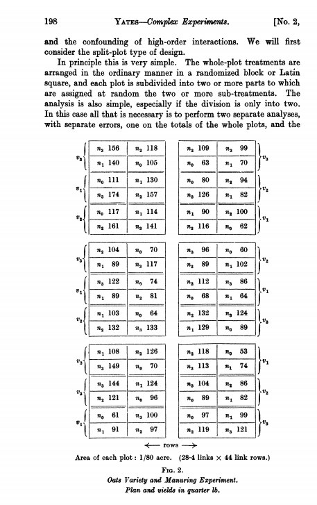
Given that I’m an unsophisticated forester and that I’d like to use data available to anyone, I’ll rely on an agricultural example (so plots are actually physical plots in the field) that goes back to Frank Yates. There are two factors (oats variety, with three levels, and fertilization, with four levels). Yates, F. (1935) Complex experiments, Journal of the Royal Statistical Society Suppl. 2, 181–247 (behind pay wall here).
The following image shows the layout of oats experiment in Yates’s paper, from a time when articles were meaty. Each of the 6 replicates is divided in to 3 main plots for oats varieties (v1, v2 and v3), while each variety was divided into four parts with different levels of fertilization (manure—animal crap—n1 to n4). Cells display yield.

Now it is time to roll up our sleeves and use some code, getting the data and fitting the same model using nlme (m1) and asreml (m2), just for the fun of it. Anyway, nlme and asreml produce exactly the same results.
We will use the oats data set that comes with MASS, although there is also an Oats data set in nlme and another version in the asreml package. (By the way, you can see a very good explanation by Bill Venables of a ‘traditional’ ANOVA analysis for a split-plot here):
library(MASS) # we get the oats data from here
library(nlme) # for lme function
library(asreml) # for asreml function. This dataset use different variable names,
# which may require renaming a dataset to use the code below

# Get the oats data set and check structure
data(oats)
head(oats)
str(oats)

# Create a main plot effect for clarity's sake
oats$MP <- oats$V

# Split-plot using NLME
m1 <- lme(Y ~ V*N,
          random = ~ 1|B/MP,
          data = oats)
summary(m1)
fixef(m1)
ranef(m1)

# Split-plot using ASReml
m2 <- asreml(Y ~ V*N,
             random = ~ B/MP,
             data = oats)
summary(m2)$varcomp
coef(m2)$fixed
coef(m2)$random

fixef(m1)
#        (Intercept)         VMarvellous            VVictory             N0.2cwt
#         80.0000000           6.6666667          -8.5000000          18.5000000
#            N0.4cwt             N0.6cwt VMarvellous:N0.2cwt    VVictory:N0.2cwt
#         34.6666667          44.8333333           3.3333333          -0.3333333
#VMarvellous:N0.4cwt    VVictory:N0.4cwt VMarvellous:N0.6cwt    VVictory:N0.6cwt
#         -4.1666667           4.6666667          -4.6666667           2.1666667

ranef(m1)
# Level: B
# (Intercept)
# I     25.421511
# II     2.656987
# III   -6.529883
# IV    -4.706019
# V    -10.582914
# VI    -6.259681
#
# Level: MP %in% B
# (Intercept)
# I/Golden.rain      2.348296
# I/Marvellous      -3.854348
# I/Victory         14.077467
# II/Golden.rain     4.298706
# II/Marvellous      6.209473
# II/Victory        -9.194250
# III/Golden.rain   -7.915950
# III/Marvellous    10.750776
# III/Victory       -6.063976
# IV/Golden.rain     5.789462
# IV/Marvellous     -7.115566
# IV/Victory        -1.001111
# V/Golden.rain      1.116768
# V/Marvellous      -9.848096
# V/Victory          3.497878
# VI/Golden.rain    -5.637282
# VI/Marvellous      3.857761
# VI/Victory        -1.316009
Now we can move to implement the Mixed Model Equations, where probably the only gotcha is the definition of the
$$\mathbf{Z}$$ matrix (incidence matrix for random effects), as both nlme and asreml use ’number of levels of the factor’ for both the main and interactions effects, which involves using the contrasts.arg argument in model.matrix().
# Variance components
varB <- 214.477
varMP <- 106.062
varR <- 177.083

# Basic vector and matrices: y, X, Z, G & R
y <- matrix(oats$Y, nrow = dim(oats)[1], ncol = 1)
X <- model.matrix(~ V*N, data = oats)
Z <- model.matrix(~ B/MP - 1, data = oats,
contrasts.arg <- list(B = contrasts(oats$B, contrasts = F),
                      MP = contrasts(oats$MP, contrasts = F)))

G <- diag(c(rep(varB, 6), rep(varMP, 18)))
R <- diag(varR, 72, 72)
Rinv <- solve(R)

# Components of C
XpX <- t(X) %*% Rinv %*% X
ZpZ <- t(Z) %*% Rinv %*% Z

XpZ <- t(X) %*% Rinv %*% Z
ZpX <- t(Z) %*% Rinv %*% X

Xpy <- t(X) %*% Rinv %*% y
Zpy <- t(Z) %*% Rinv %*% y

# Building C * [b a] = RHS
C <- rbind(cbind(XpX, XpZ),
           cbind(ZpX, ZpZ + solve(G)))
RHS <- rbind(Xpy, Zpy)

blup <- solve(C, RHS)
blup

# [,1]
# (Intercept)          80.0000000
# VMarvellous           6.6666667
# VVictory             -8.5000000
# N0.2cwt              18.5000000
# N0.4cwt              34.6666667
# N0.6cwt              44.8333333
# VMarvellous:N0.2cwt   3.3333333
# VVictory:N0.2cwt     -0.3333333
# VMarvellous:N0.4cwt  -4.1666667
# VVictory:N0.4cwt      4.6666667
# VMarvellous:N0.6cwt  -4.6666667
# VVictory:N0.6cwt      2.1666667
# BI                   25.4215578
# BII                   2.6569919
# BIII                 -6.5298953
# BIV                  -4.7060280
# BV                  -10.5829337
# BVI                  -6.2596927
# BI:MPGolden.rain      2.3482656
# BII:MPGolden.rain     4.2987082
# BIII:MPGolden.rain   -7.9159514
# BIV:MPGolden.rain     5.7894753
# BV:MPGolden.rain      1.1167834
# BVI:MPGolden.rain    -5.6372811
# BI:MPMarvellous      -3.8543865
# BII:MPMarvellous      6.2094778
# BIII:MPMarvellous    10.7507978
# BIV:MPMarvellous     -7.1155687
# BV:MPMarvellous      -9.8480945
# BVI:MPMarvellous      3.8577740
# BI:MPVictory         14.0774514
# BII:MPVictory        -9.1942649
# BIII:MPVictory       -6.0639747
# BIV:MPVictory        -1.0011059
# BV:MPVictory          3.4978963
# BVI:MPVictory        -1.3160021
Not surprisingly, we get the same results, except that we start assuming the variance components from the previous analyses, so we can avoid implementing the code for restricted maximum likelihood estimation as well. By the way, given that
$$\mathbf{R}^{-1}$$is in all terms it can be factored out from the MME, leaving terms like
$$\mathbf{X}' \mathbf{X}$$, i.e. without
$$\mathbf{R}^{-1}$$, making for simpler calculations. In fact, if you drop the
$$\mathbf{R}^{-1}$$it is easier to see what is going on in the different components of the
$$\mathbf{C}$$matrix. For example, print
$$\mathbf{X}' \mathbf{X}$$and you’ll get the sum of observations for the overall mean and for each of the levels of the fixed effect factors. Give it a try with the other submatrices too!
XpXnoR <- t(X) %*% X
XpXnoR
#                    (Intercept) VMarvellous VVictory N0.2cwt N0.4cwt N0.6cwt
#(Intercept)                  72          24       24      18      18      18
#VMarvellous                  24          24        0       6       6       6
#VVictory                     24           0       24       6       6       6
#N0.2cwt                      18           6        6      18       0       0
#N0.4cwt                      18           6        6       0      18       0
#N0.6cwt                      18           6        6       0       0      18
#VMarvellous:N0.2cwt           6           6        0       6       0       0
#VVictory:N0.2cwt              6           0        6       6       0       0
#VMarvellous:N0.4cwt           6           6        0       0       6       0
#VVictory:N0.4cwt              6           0        6       0       6       0
#VMarvellous:N0.6cwt           6           6        0       0       0       6
#VVictory:N0.6cwt              6           0        6       0       0       6
#                    VMarvellous:N0.2cwt VVictory:N0.2cwt VMarvellous:N0.4cwt
#(Intercept)                           6                6                   6
#VMarvellous                           6                0                   6
#VVictory                              0                6                   0
#N0.2cwt                               6                6                   0
#N0.4cwt                               0                0                   6
#N0.6cwt                               0                0                   0
#VMarvellous:N0.2cwt                   6                0                   0
#VVictory:N0.2cwt                      0                6                   0
#VMarvellous:N0.4cwt                   0                0                   6
#VVictory:N0.4cwt                      0                0                   0
#VMarvellous:N0.6cwt                   0                0                   0
#VVictory:N0.6cwt                      0                0                   0
#                    VVictory:N0.4cwt VMarvellous:N0.6cwt VVictory:N0.6cwt
#(Intercept)                        6                   6                6
#VMarvellous                        0                   6                0
#VVictory                           6                   0                6
#N0.2cwt                            0                   0                0
#N0.4cwt                            6                   0                0
#N0.6cwt                            0                   6                6
#VMarvellous:N0.2cwt                0                   0                0
#VVictory:N0.2cwt                   0                   0                0
#VMarvellous:N0.4cwt                0                   0                0
#VVictory:N0.4cwt                   6                   0                0
#VMarvellous:N0.6cwt                0                   6                0
#VVictory:N0.6cwt                   0                   0                6
I will leave it here and come back to this problem as soon as I can.
† Incidentally, a lot of the theoretical development was supported by Shayle Searle (a Kiwi statistician and Henderson’s colleague in Cornell University).