Covariance structures

In most mixed linear model packages (e.g. asreml, lme4, nlme, etc) one needs to specify only the model equation (the bit that looks like y ~ factors...) when fitting simple models. We explicitly say nothing about the covariances that complete the model specification. This is because most linear mixed model packages assume that, in absence of any additional information, the covariance structure is the product of a scalar (a variance component) by a design matrix. For example, the residual covariance matrix in simple models is R = I σ_e², or the additive genetic variance matrix is G = A σ_a² (where A is the numerator relationship matrix), or the covariance matrix for a random effect f with incidence matrix Z is Z‘ Z σ_f².

However, there are several situations when analyses require a more complex covariance structure, usually a direct sum or a Kronecker product of two or more matrices. For example, an analysis of data from several sites might consider different error variances for each site, that is R = Σd R_i, where Σd represents a direct sum and R_i is the residual matrix for site i.

Other example of a more complex covariance structure is a multivariate analysis in a single site (so the same individual is assessed for two or more traits), where both the residual and additive genetic covariance matrices are constructed as the product of two matrices. For example, R = I ⊗ R₀, where I is an identity matrix of size number of observations, ⊗ is the Kronecker product (do not confuse with a plain matrix multiplication) and R₀ is the error covariance matrix for the traits involved in the analysis. Similarly, G = A ⊗ G₀ where all the matrices are as previously defined and G₀ is the additive covariance matrix for the traits.

Some structures are easier to understand (at least for me) if we express a covariance matrix (M) as the product of a correlation matrix (C) pre- and post-multiplied by a diagonal matrix (D) containing standard deviations for each of the traits (M = D C D). That is:

\(
M = \left [
\begin{array}{cccc}
v_{11}& c_{12}& c_{13}& c_{14} \
c_{21}& v_{22}& c_{23}& c_{24} \
c_{31}& c_{32}& v_{33}& c_{34} \
c_{41}& c_{42}& c_{43}& v_{44}
\end{array}
\right ]\)
\(
C = \left [
\begin{array}{cccc}
\n1& r_{12}& r_{13}& r_{14} \
r_{21}& 1& r_{23}& r_{24} \
r_{31}& r_{32}& 1& r_{34} \
r_{41}& r_{42}& r_{43}& 1
\end{array}
\right ]\)
\(
D = \left [
\begin{array}{cccc}
s_{11}& 0& 0& 0 \
\n0& s_{22}& 0& 0 \
\n0& 0& s_{33}& 0 \
\n0& 0& 0& s_{44}
\end{array}
\right ]\)

where the v are variances, the r correlations and the s standard deviations.

If we do not impose any restriction on M, apart from being positive definite (p.d.), we are talking about an unstructured matrix (us() in asreml-R parlance). Thus, M or C can take any value (as long as it is p.d.) as it is usual when analyzing multiple trait problems.

There are cases when the order of assessment or the spatial location of the experimental units create patterns of variation, which are reflected by the covariance matrix. For example, the breeding value of an individual i observed at time j (a_ij) is a function of genes involved in expression at time j – k (a_ij-k), plus the effect of genes acting in the new measurement (α_j), which are considered independent of the past measurement a_ij = ρ_jk a_ij-k + α_j, where ρ_jk is the additive genetic correlation between measures j and k.

Rather than using a different correlation for each pair of ages, it is possible to postulate mechanisms which model the correlations. For example, an autoregressive model (ar() in asreml-R lingo), where the correlation between measurements j and k is r^|j-k|. In this model M = D C_AR D, where C_AR (for equally spaced assessments) is:
\(
C_{AR} = \left [
\begin{array}{cccc}
\n1 & r^{|t_2-t_1|} & \ldots & r^{|t_m-t_1|}\
r^{|t_2-t_1|} & 1 & \ldots & r^{|t_m-t_2|}\
\vdots & \vdots & \ddots & \vdots \
r^{|t_m-t_1|} & r^{|t_m-t_2|} & \ldots & 1
\end{array}
\right ]\)

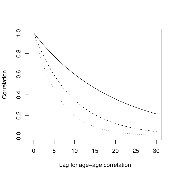
Assuming three different autocorrelation coefficients (0.95 solid line, 0.90 dashed line and 0.85 dotted line) we can get very different patterns with a few extra units of lag, as shown in the following graph:

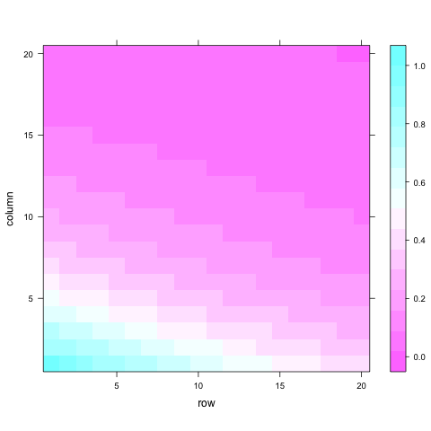
A model including this structure will certainly be more parsimonious (economic on terms of number of parameters) than one using an unstructured approach. Looking at the previous pattern it is a lot easier to understand why they are called ‘structures’. A similar situation is considered in spatial analysis, where the ‘independent errors’ assumption of typical analyses is relaxed. A common spatial model will consider the presence of autocorrelated residuals in both directions (rows and columns). Here the level of autocorrelation will depend on distance between trees rather than on time. We can get an idea of how separable processes look like using this code:

# Separable row col autoregressive process
car2 <- function(dim, rhor, rhoc) {
  M <- diag(dim)
  rhor^(row(M) - 1) * rhoc^(col(M) - 1)
}

library(lattice)
levelplot(car2(20, 0.95, 0.85))

This correlation matrix can then be multiplied by a spatial residual variance to obtain the covariance and we can add up a spatially independent residual variance.

Much more detail on code notation for covariance structures can be found, for example, in the ASReml-R User Guide (PDF, chapter 4), for nlme in Pinheiro and Bates's Mixed-effects models in S and S-plus (link to Google Books, chapter 5.3) and in Bates's draft book for lme4 in chapter 4.