Until today all the posts in this blog have used a frequentist view of the world. I have a confession to make: I have an ecumenical view of statistics and I do sometimes use Bayesian approaches in data analyses. This is not quite one of those “the truth will set you free” moments, but I’ll show that one could almost painlessly repeat some of the analyses I presented before using MCMC.
Continue reading
Category: linear models (Page 3 of 4)
I swear there was a point in writing an introduction to covariance structures: now we can start joining all sort of analyses using very similar notation. In a previous post I described simple (even simplistic) models for a single response variable (or ‘trait’ in quantitative geneticist speak). The R code in three R packages (asreml-R, lme4 and nlme) was quite similar and we were happy-clappy with the consistency of results across packages. The curse of the analyst/statistician/guy who dabbles in analyses is the idea that we can always fit a nicer model and—as both Bob the Builder and Obama like to say—yes, we can.
Continue reading
Last Wednesday I had a meeting with the folks of the New Zealand Drylands Forest Initiative in Blenheim. In addition to sitting in a conference room and having nice sandwiches we went to visit one of our progeny trials at Cravens. Plantation forestry trials are usually laid out following a rectangular lattice defined by rows and columns. The trial follows an incomplete block design with 148 blocks and is testing 60 Eucalyptus bosistoana families. A quick look at survival shows an interesting trend: the bottom of the trial was much more affected by frost than the top.
Continue reading
In a previous post I summarily described our options for (generalized to varying degrees) linear mixed models from a frequentist point of view: nlme, lme4 and ASReml-R†, followed by a quick example for a split-plot experiment.
But who is really happy with a toy example? We can show a slightly more complicated example assuming that we have a simple situation in breeding: a number of half-sib trials (so we have progeny that share one parent in common), each of them established following a randomized complete block design, analyzed using a ‘family model’. That is, the response variable (dbh: tree stem diameter assessed at breast height—1.3m from ground level) can be expressed as a function of an overall mean, fixed site effects, random block effects (within each site), random family effects and a random site-family interaction. The latter provides an indication of genotype by environment interaction.
Continue reading
A substantial part of my job has little to do with statistics; nevertheless, a large proportion of the statistical side of things relates to applications of linear mixed models. The bulk of my use of mixed models relates to the analysis of experiments that have a genetic structure.
A brief history of time
At the beginning (1992-1995) I would use SAS (first proc glm, later proc mixed), but things started getting painfully slow and limiting if one wanted to move into animal model BLUP. At that time (1995-1996), I moved to DFREML (by Karen Meyer, now replaced by WOMBAT) and AIREML (by Dave Johnson, now defunct—the program I mean), which were designed for the analysis of animal breeding progeny trials, so it was a hassle to deal with experimental design features. At the end of 1996 (or was it the beginning of 1997?) I started playing with ASReml (programed by Arthur Gilmour mostly based on theoretical work by Robin Thompson and Brian Cullis). I was still using SAS for data preparation, but all my analyses went through ASReml (for which I wrote the cookbook), which was orders of magnitude faster than SAS (and could deal with much bigger problems). Around 1999, I started playing with R (prompted by a suggestion from Rod Ball), but I didn’t really use R/S+ often enough until 2003. At the end of 2005 I started using OS X and quickly realized that using a virtual machine or dual booting was not really worth it, so I dropped SAS and totally relied on R in 2009.
Continue reading


