Updating and expanding New Zealand school data
In two previous posts I put together a data set and presented some exploratory data analysis on school achievement for national standards. After those posts I exchanged emails with a few people about the sources of data and Jeremy Greenbrook-Held pointed out Education Counts as a good source of additional variables, including number of teachers per school and proportions for different ethnic groups.
The code below call three files: Directory-Schools-Current.csv, teacher-numbers.csv and SchoolReport_data_distributable.csv, which you can download from the links.
options(stringsAsFactors = FALSE)

library(ggplot2)

# Reading School directory and dropping some address information
# for 2012 obtained from here:
# http://www.educationcounts.govt.nz/directories/list-of-nz-schools
directory <- read.csv('Directory-Schools-Current.csv')
directory <- subset(directory, select = -1*c(3:9, 11:13))

# Reading teacher numbers for 2011 obtained from here:
# http://www.educationcounts.govt.nz/statistics/schooling/teaching_staff
teachers <- read.csv('teacher-numbers.csv')

# Reading file obtained from stuff.co.nz obtained from here:
# http://schoolreport.stuff.co.nz/index.html
fairfax <- read.csv('SchoolReport_data_distributable.csv')

# Merging directory and teachers info
standards <- merge(directory, teachers, by = 'school.id', all.x = TRUE)

# Checking that the school names match
# This shows ten cases, some of them obviously the same school
# e.g. Epsom Girls Grammar School vs Epsom Girls' Grammar School
tocheck <- subset(standards, school.name.x != school.name.y)
tocheck[, c(1:2, 29)]
#school.id                          school.name.x                  school.name.y
#61          64             Epsom Girls Grammar School    Epsom Girls' Grammar School
#125        135                     Fraser High School  Hamilton's Fraser High School
#362        402                      Waiau Area School    Tuatapere Community College
#442        559                        Te Wainui a Rua           Whanganui Awa School
#920       1506 St Michael's Catholic School (Remuera)  St Michael's School (Remuera)
#929       1515                      Sunnyhills School             Sunny Hills School
#985       1573                     Willow Park School              Willowpark School
#1212      1865               Te Wharekura o Maniapoto         Te Wharekura o Oparure
#1926      2985          Sacred Heart Cathedral School Sacred Heart School (Thorndon)
#2266      3554                         Waitaha School        Waitaha Learning Centre

# Merging now with fairfax data
standards <- merge(standards, fairfax,
                   by = 'school.id', all.x = TRUE)

# Four schools have a different name
tocheck2 <- subset(standards, school.name.x != school.name)
tocheck2[, c(1:2, 32)]
#school.id                          school.name.x                   school.name
#920       1506 St Michael's Catholic School (Remuera) St Michael's School (Remuera)
#929       1515                      Sunnyhills School            Sunny Hills School
#985       1573                     Willow Park School             Willowpark School
#2266      3554                         Waitaha School       Waitaha Learning Centre

# Checking the original spreadsheets it seems that, despite
# the different name they are the same school (at least same
# city)

# Now start dropping a few observations that are of no use
# for any analysis; e.g. schools without data
standards <- subset(standards, !is.na(reading.WB))

# Dropping school 498 Te Aho o Te Kura Pounamu Wellington
# http://www.tekura.school.nz/
# It is a correspondence school without decile information
standards <- subset(standards, school.id != 498)

# Converting variables to factors
standards$decile <- factor(standards$decile)
standards$school.type <- factor(standards$school.type)
standards$education.region <- factor(standards$education.region,
                                     levels = c('Northern', 'Central North', 'Central South', 'Southern'))

# Removing 8 special schools
standards <- subset(standards, as.character(school.type) != 'Special School')
standards$school.type <- standards$school.type[drop = TRUE]

# Saving file for Eric
# write.csv(standards, 'standardsUpdated.csv',
#          row.names = FALSE, quote = FALSE)

# Create performance groups
standards$math.OK <- with(standards, math.At + math.A)
standards$reading.OK <- with(standards, reading.At + reading.A)
standards$writing.OK <- with(standards, writing.At + writing.A)

# Creating a few proportions
standards$prop.euro <- with(standards, european/total.roll)
standards$prop.maori <- with(standards, maori/total.roll)
standards$prop.pacific <- with(standards, pacific.island/total.roll)
standards$prop.asian <- with(standards, asian/total.roll)
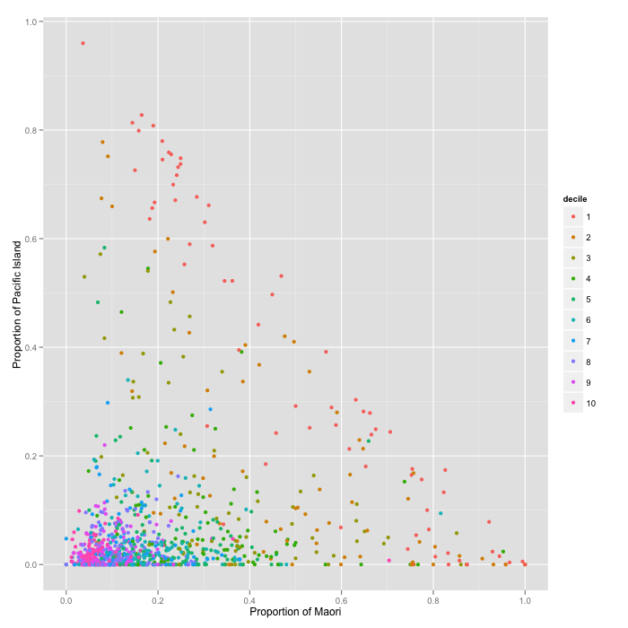
This updated data set is more comprehensive but it doesn’t change the general picture presented in my previous post beyond the headlines. Now we can get some cool graphs to point out the obvious, for example the large proportion of Maori and Pacific Island students in low decile schools:
qplot(prop.maori, prop.pacific,
      data = standards, color = decile,
      xlab = 'Proportion of Maori',
      ylab = 'Proportion of Pacific Island')

I have avoided ‘proper’ statistical modeling because i- there is substantial uncertainty in the data and ii- the national standards for all schools (as opposed to only 1,000 schools) will be released soon; we do’t know if the published data are a random sample. In any case, a quick linear model fitting the proportion of students that meet reading standards (reading.OK) as a function of decile and weighted by total school roll—to account for the varying school sizes—will explain roughly 45% of the observed variability on reading achievement.
m1 <- lm(reading.OK ~ decile,
         data = standards,
         weights = total.roll)
summary(m1)

# Coefficients:
#   Estimate Std. Error t value Pr(>|t|)
# (Intercept)  0.56164    0.01240  45.278  < 2e-16 ***
#   decile2      0.06238    0.01769   3.527 0.000439 ***
#   decile3      0.10890    0.01749   6.225 7.07e-10 ***
#   decile4      0.16434    0.01681   9.774  < 2e-16 ***
#   decile5      0.18579    0.01588  11.697  < 2e-16 ***
#   decile6      0.22849    0.01557  14.675  < 2e-16 ***
#   decile7      0.25138    0.01578  15.931  < 2e-16 ***
#   decile8      0.24849    0.01488  16.701  < 2e-16 ***
#   decile9      0.28861    0.01492  19.347  < 2e-16 ***
#   decile10     0.31074    0.01439  21.597  < 2e-16 ***
#
# Residual standard error: 1.594 on 999 degrees of freedom
# (1 observation deleted due to missingness)
# Multiple R-squared: 0.4548,  Adjusted R-squared: 0.4499
# F-statistic: 92.58 on 9 and 999 DF,  p-value: < 2.2e-16
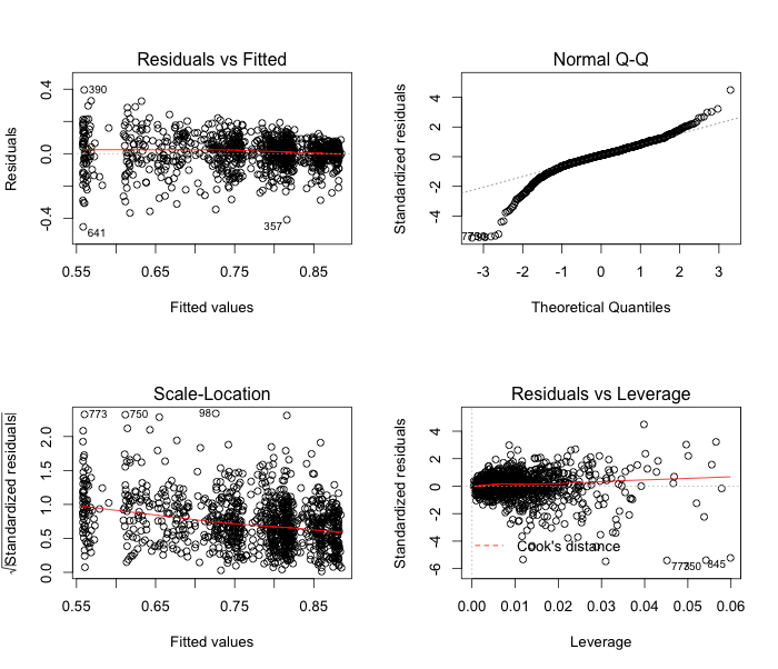
Model fit has a few issues with distribution of residuals, we should probably use a power transformation for the response variable, but I wouldn’t spend much more time before getting the full data for national standards.
par(mfrow = c(2, 2))
plot(m1)
par(mfrow = c(1, 1))

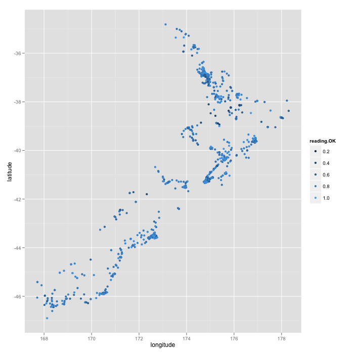
Bonus plot: map of New Zealand based on school locations, colors depicting proportion of students meeting reading national standards.
qplot(longitude, latitude,
      data = standards, color = reading.OK)

P.S. 2012-09-26 16:01. The simple model above could be fitted taking into account the order of the decile factor (using ordered()) or just fitting linear and quadratic terms for a numeric expression of decile. Anyway, that would account for 45% of the observed variability.
m1d <- lm(reading.OK ~ as.numeric(decile) + I(as.numeric(decile)^2),
          data = standards, weights = total.roll)
summary(m1d)

#Coefficients:
#                          Estimate Std. Error t value Pr(>|t|)
#(Intercept)              0.5154954  0.0136715  37.706  < 2e-16 ***
#as.numeric(decile)       0.0583659  0.0051233  11.392  < 2e-16 ***
#I(as.numeric(decile)^2) -0.0023453  0.0004251  -5.517 4.39e-08 ***
#---
#Residual standard error: 1.598 on 1006 degrees of freedom
#  (1 observation deleted due to missingness)
#Multiple R-squared: 0.4483,    Adjusted R-squared: 0.4472
#F-statistic: 408.8 on 2 and 1006 DF,  p-value: < 2.2e-16
P.S. 2012-09-26 18:17. Eric Crampton has posted preliminary analyses based on this dataset in Offsetting Behaviour.