Evolving notes, images and sounds by Luis Apiolaza

My take on the USA versus Western Europe comparison of GM corn

A few days ago I came across Jack Heinemann and collaborators’ article (Sustainability and innovation in staple crop production in the US Midwest, Open Access) comparing the agricultural sectors of USA and Western Europe. While the article is titled around the word sustainability, the main comparison stems from the use of Genetically Modified crops in USA versus the absence of them in Western Europe.

I was curious about part of the results and discussion which, in a nutshell, suggest that “GM cropping systems have not contributed to yield gains, are not necessary for yield gains, and appear to be eroding yields compared to the equally modern agroecosystem of Western Europe”. The authors relied on several crops for the comparison (Maize/corn, rapeseed/canolasee P.S.6, soybean and cotton); however, I am going to focus on a single one (corn) for two reasons: 1. I can’t afford a lot of time for blog posts when I should be preparing lectures and 2. I like eating corn.

When the authors of the paper tackled corn the comparison was between the USA and Western Europe, using the United Nations definition of Western Europe (i.e. Austria, Belgium, France, Germany, Liechtenstein, Luxembourg, Monaco, Netherlands, Switzerland). Some large European corn producers like Italy are not there because of the narrow definition of Western.

I struggled with the comparison used by the authors because, in my opinion, there are potentially so many confounded effects (different industry structures, weather, varieties, etc.) that it can’t provide the proper counterfactual for GM versus non-GM crops. Anyway, I decided to have a look at the same data to see if I would reach the same conclusions. The article provides a good description of where the data came from, as well as how the analyses were performed. Small details to match exactly the results were fairly easy to figure out. I downloaded the FAO corn data (3.7 MB csv file) for all countries (so I can reuse the code and data later for lectures and assignments). I then repeated the plots using the following code:

# Default directory
setwd('~/Dropbox/quantumforest')

# Required packages
library(ggplot2)
library(labels)

# Reading FAO corn data
FAOcorn <- read.csv('FAOcorn.csv')

# Extracting Area
FAOarea <- subset(FAOcorn, Element == 'Area Harvested',
                  select = c('Country', 'Year', 'Value'))

names(FAOarea)[3] <- 'Area'

# and production
FAOprod <- subset(FAOcorn, Element == 'Production',
                  select = c('Country', 'Year', 'Value'))

names(FAOprod)[3] <- 'Production'

# to calculate yield in hectograms
FAOarea <- merge(FAOarea, FAOprod, by = c('Country', 'Year'))
FAOarea$Yield <- with(FAOarea, Production/Area*10000)

# Subsetting only the countries of interest (and years to match paper)
FAOarticle <- subset(FAOarea, Country == 'United States of America' | Country == 'Western Europe')

# Plot with regression lines
ggplot(FAOarticle, aes(x = Year, y = Yield, color = Country)) +
  geom_point() + stat_smooth(method = lm, fullrange = TRUE, alpha = 0.1) +
  scale_y_continuous('Yield [hectograms/ha]', limits = c(0, 100000), labels = comma) +
  theme(legend.position="top")
Figure 1. Corn yield per year for USA and Western Europe (click to enlarge).

Figure 1. Corn yield per year for USA and Western Europe (click to enlarge).

I could obtain pretty much the same regression model equations as in the article by expressing the years as deviation from 1960 as in:

# Expressing year as a deviation from 1960, so results
# match paper
FAOarticle$NewYear <- with(FAOarticle, Year - 1960)

usa.lm <- lm(Yield ~ NewYear, data = FAOarticle,
             subset = Country == 'United States of America')
summary(usa.lm)

#Call:
#lm(formula = Yield ~ NewYear, data = FAOarticle, subset = Country ==
#    "United States of America")
#
#Residuals:
#     Min       1Q   Median       3Q      Max
#-18435.4  -1958.3    338.3   3663.8  10311.0
#
#Coefficients:
#            Estimate Std. Error t value Pr(>|t|)
#(Intercept) 38677.34    1736.92   22.27|t|)
#(Intercept) 31510.14    1665.90   18.91

Heinemann and collaborators then point out the following:

...the slope in yield increase by year is steeper in W. Europe (y = 1344.2x + 31512, R² = 0.92084) than the United States (y = 1173.8x + 38677, R² = 0.89093) from 1961 to 2010 (Figure 1). This shows that in recent years W. Europe has had similar and even slightly higher yields than the United States despite the latter's use of GM varieties.

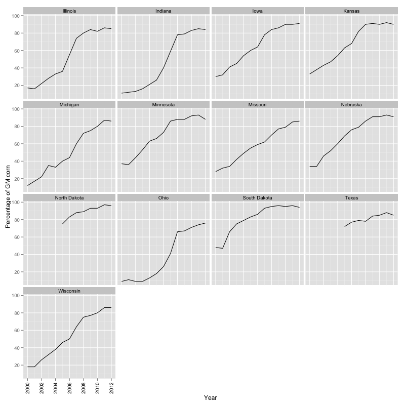
However, that interpretation using all data assumes that both 'countries' are using GMO all the time. An interesting thing is that USA and Western Europe were in different trends already before the introduction of GM corn. We can state that because we have some idea of when GM crops were introduced in the USA. This information is collected by the US Department of Agriculture in their June survey to growers and made publicly available at the State level (GMcornPenetration.csv):
cornPenetration <- read.csv('GMcornPenetration.csv')

ggplot(cornPenetration, aes(x = Year, y = PerAllGM)) + geom_line() + facet_wrap(~ State) +
  scale_y_continuous('Percentage of GM corn') +
  theme(axis.text.x  = theme_text(angle=90))
GM corn percentage by state in the USA.

Figure 2. GM corn percentage by state in the USA (click to enlarge).

This graph tells us that by the year 2000 the percentage of planted corn was way below 50% in most corn producing states (in fact, it was 25% at the country level). From that time on we have a steady increase reaching over 80% for most states by 2008. Given this, it probably makes sense to assume that, at the USA level, yield reflects non-GM corn until 1999 and progressively reflects the effect of GM genotypes from 2000 onwards. This division is somewhat arbitrary, but easy to implement.

We can repeat the previous analyzes limiting the data from 1961 until, say, 1999:

usa.lm2 <- lm(Yield ~ NewYear, data = FAOarticle,
              subset = Country == 'United States of America' & Year < 2000)
summary(usa.lm2)

#Call:
#lm(formula = Yield ~ NewYear, data = FAOarticle, subset = Country ==
#    "United States of America" & Year < 2000)
#
#Residuals:
#   Min     1Q Median     3Q    Max
#-17441  -2156   1123   3989   9878
#
#Coefficients:
#            Estimate Std. Error t value Pr(>|t|)
#(Intercept) 39895.57    2084.81   19.14  < 2e-16 ***
#NewYear      1094.82      90.84   12.05 2.25e-14 ***
#---
#Signif. codes:  0 ‘***’ 0.001 ‘**’ 0.01 ‘*’ 0.05 ‘.’ 0.1 ‘ ’ 1
#
#Residual standard error: 6385 on 37 degrees of freedom
#Multiple R-squared:  0.797,	Adjusted R-squared:  0.7915
#F-statistic: 145.2 on 1 and 37 DF,  p-value: 2.245e-14

weu.lm2 <- lm(Yield ~ NewYear, data = FAOarticle,
              subset = Country == 'Western Europe' & Year < 2000)
summary(weu.lm2)

#Call:
#lm(formula = Yield ~ NewYear, data = FAOarticle, subset = Country ==
#    "Western Europe" & Year < 2000)
#
#Residuals:
#   Min     1Q Median     3Q    Max
#-10785  -3348    -34   3504  11117
#
#Coefficients:
#            Estimate Std. Error t value Pr(>|t|)
#(Intercept) 29802.17    1813.79   16.43

These analyses indicate that Western Europe started with a lower yield than the USA (29,802.17 vs 39,895.57 hectograms/ha) and managed to increase yield much more quickly (1,454.48 vs 1,094.82 hectograms/ha per year) before any use of GM corn by the USA. Figure 1 shows a messy picture because there are numerous factors affecting yield each year (e.g. weather has a large influence). We can take averages for each decade and see how the two 'countries' are performing:

# Aggregating every decade.
# 2013-07-05 20:10 NZST I fixed the aggregation because it was averaging yields rather
# calculating total production and area for the decade and then calculating average yield
# Discussion points are totally valid
FAOarticle$Decade <- cut(FAOarticle$Year,
                         breaks = seq(1959, 2019, 10),
                         labels = paste(seq(1960, 2010, 10), 's', sep = ''))

decadeProd <- aggregate(Production ~ Country + Decade,
                        data = FAOarticle,
                        FUN = sum)

decadeArea <- aggregate(Area ~ Country + Decade,
                        data = FAOarticle,
                        FUN = sum)

decadeYield <- merge(decadeProd, decadeArea, by = c('Country', 'Decade'))
decadeYield$Yield <- with(decadeYield, Production/Area*10000)

ggplot(decadeYield, aes(x = Decade, y = Yield, fill = Country)) +
  geom_bar(stat = 'identity', position = 'dodge') +
  scale_y_continuous('Yield [hectograms/ha]', expand = c(0, 0)) +
  theme(legend.position="top")
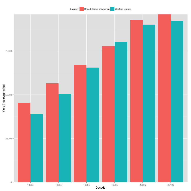
Figure 3. Corn yield by decade (click to enlarge).

Figure 3. Corn yield by decade (click to enlarge).

This last figure requires more attention. We can again see that Western Europe starts with lower yields than the USA; however, it keeps on increasing those yields faster than USA, overtaking it during the 1990s. Again, all this change happened while both USA and Western Europe were not using GM corn. The situation reverses in the 2000s, when the USA overtakes Western Europe, while the USA continuously increased the percentage of GM corn. The last bar in Figure 3 is misleading because it includes a single year (2010) and we know that yields in USA went down in 2011 and 2012, affected by a very large drought (see Figure 4).

At least when looking at corn, I can't say (with the same data available to Heinemann) that there is no place or need for GM genotypes. I do share some of his concerns with respect to the low level of diversity present in staple crops but, in contrast to his opinion, I envision a future for agriculture that includes large-scale operations (either GM or no-GM), as well as smaller operations (including organic ones). I'd like to finish with some optimism looking further back to yield, because the USDA National Agricultural Statistics Service keeps yield statistics for corn since 1866(!) (csv file), although it uses bizarre non-metric units (bushels/acre). As a metric boy, I converted to kilograms per hectare (multiplying by 62.77 from this page) and then to hectograms (100 g) multiplying by 10.

# Reading NASS corn data
NASS <- read.csv('NASScorn.csv')

# Conversion to sensical units (see Iowa State Extension article)
# http://www.extension.iastate.edu/agdm/wholefarm/html/c6-80.html
NASS$Yield <- with(NASS, Value*62.77*10)

# Average by decade
NASS$Decade <- cut(NASS$Year,
                   breaks = seq(1859, 2019, 10),
                   labels = paste(seq(1860, 2010, 10), 's', sep = ''))

oldYield <- aggregate(Yield ~ Decade, data = NASS, FUN = mean)

# Plotting
ggplot(oldYield, aes(x = Decade, y = Yield)) +
  geom_bar(stat = 'identity') +
  scale_y_continuous('Yield [hectograms]', expand = c(0, 0))
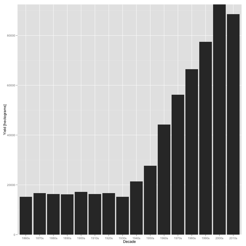
Historic average yield per decade for USA (click to enlarge).

Figure 4. Historic average yield per decade for USA (click to enlarge).

It is interesting to see that there was little change until the 1940s, with the advent of the Green Revolution (modern breeding techniques, fertilization, pesticides, etc.). The 2010s decade in Figure 4 includes 2010, 2011 and 2012, with the last two years reflecting extensive droughts. Drought tolerance is one of the most important traits in modern breeding programs.
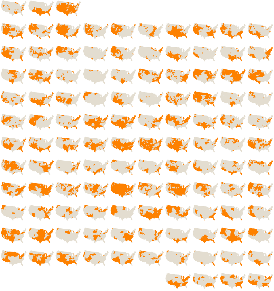
Drought’s Footprint map produced by The New York Times (click on graph to view larger version in the NYT).

Drought’s Footprint map produced by The New York Times (click on graph to view larger version in the NYT). This can help to understand the Decade patterns in previous figures.

While Prof. Heinemann and myself work for the same university I don't know him in person.

P.S. Did you know that Norman Borlaug (hero of mine) studied forestry?
P.S.2 Time permitting I'll have a look at other crops later. I would have liked to test a regression with dummy variables for corn to account for pre-2000 and post-1999, but there are not yet many years to fit a decent model (considering natural variability between years). We'll have to wait for that one.
P.S.3 I share some of Heinemann's concerns relating to subsidies and other agricultural practices.
P.S.4 In case anyone is interested, I did write about a GM-fed pigs study not long ago.
P.S.5 2013-07-05 20:10 NZST. I updated Figures 1 and 3 to clearly express that yield was in hectograms/ha and recalculated average decade yield because it was originally averaging yields rather calculating total production and area for the decade and then calculating average yield. The discussion points I raised are still completely valid.
P.S.6 2013-07-07 11:30 NZST. The inclusion of Canadian canola does not make any sense because, as far as I know, Canada is not part of Western Europe or the US Midwest. This opens the inclusion of crops from any origin as far as the results are convenient for one's argument.
P.S.7 2014-08-06 13:00 NZST My comment was expanded and published in the journal (or here for HTML version with comments on the authors' reply to my comment.

22 Comments

  1. Michael Manti

    Why is the comparison in terms of total yield rather than in yield per farmed area?

    • Luis

      I’m attempting to reproduce the analyses performed by the authors. I’d appreciate if you can explain the distinction you make; AFAIK yield was calculated as total production divided by planted area.

  2. Timberati

    Nice analysis Luis.

    I had forgotten that Norman Borlaug (a hero of mine too) had studied forestry (perhaps the only thing I have in common with the great man).

    What struck me is the change that occurs in the 1940’s. Of course WWII could have affected some of the output (the call to increase output for the war effort put more land under cultivation, I suspect), but it appears that mechanization (no need to pasture draft animals frees up land for crop growing), synthetic fertilization and pesticides, and probably better breeding techniques had quite a bit to do with the rise.

    • Ben Edge

      Adoption of hybrid corn was probably hindered by the Great Depression and Dust Bowl years during the 30s and picked up with the demand created by WWII and the return to normalcy after the war in the late 40s. Once hybrids took off, there was a big jump.

  3. Michael P. Manti

    I was confused by the labeling of the y-axes, which indicates mass (hectograms) rather than mass per area.

    • Luis

      I’ll fix that this (NZ) afternoon. The units are a bit weird; I’d normally use tons/ha or kg/ha, but I’m matching the paper.

  4. Robert Young

    GM plants are mostly about corporate control of the food supply, not productivity. The recent Monsanto cases are, well, case in point. This is an insidious, creeping fascism (read the wiki on Mussolini, if you disagree). Monsanto asserts it can control the seed supply, and so far gets its way. Here: http://www.farmtoconsumer.org/news_wp/?p=7764 is a recent report. While your graphing isn’t about the motivation of GM, said motivation outweighs the graphs.

    In any case, the only way to really know is a classic Fisher experiment.

    • Robert Young

      Two points I forgot, and I find no way to edit; sorry about that.
      1) some years ago I read an interview with farmers about the “Green Revolution” effect on farming. One said, paraphrasing, “There’s nothing left in the soil. It’s just dirt to hold up the plants. Fertilizers and poisons do it all.”
      2) Monsanto, at least, builds GM seeds resistant to its own poisons. The same for the rest.

      As to whether drought resistance has, or even can, be engineered, again a link: http://www.motherjones.com/tom-philpott/2012/01/monsanto-gmo-drought-tolerant-corn

      It’s increasingly unclear whether, from the Green Revolution forward, we’ve built an even less sustainable agriculture. To get the answers sounds like a job for Statistician Man (red Sigma emblazoned on rows of green and brown).

      • Luis

        Obviously something is sustainable if one can keep on doing it. There are parts of our agricultural practices that work well and parts that don’t. There are applications of agrochemicals that are positive and some that aren’t. Rather than using blanket statements, in my work (and I am a breeder by training, by the way) I use available data to improve management decisions. The data here do not tell a bad story for GM crops and I can keep on going with other parts of the paper that are highly misleading based on data, not slogans.

        There are plenty of sites where people can say what they ‘feel’ about a topic. This is not one of them; as stated in The Elements of Statistical Learning ‘In God we trust, all others bring data [and code]’.

    • Luis

      If you don’t want to have only large corporations controlling GM crops reduce the level of regulation for them: that’s crippling the entrance of new smaller competitors. I’m interested in the technical claims of the article, which I think are wrong and make data and code available as evidence to support my comments. Your points are ideological.

  5. Nick

    Where can I find the labels package? Is it on R-cran?

    • Luis

      Yes, it is in CRAN. You can install it from the menus in your version of R. The only use in my code is to add commas to the labels.

  6. Robert Young

    — The inclusion of Canadian canola does not make any sense because, as far as I know, Canada is not part of Western Europe or the US Midwest.

    Makes perfect sense, if you’re interested in the response of a contiguous growing region (under similar/identical conditions): it’s called The Great Plains, and spans the US/Canadian border; the Midwest is only the US.

    “In contrast, the adoption of GM soybeans, maize, rapeseed and cotton in the North American agroecosystem has reached near saturation. According to the industry site GMO Compass (Anon 2011), the proportion of GM rapeseed reached 82% in the United States by 2007 and 95% in Canada by 2009.”

    • Robert Young

      *isn’t* dang fingers

    • Luis

      The paper is entitled ‘Sustainability and innovation in staple crop production in the US Midwest‘. If the authors are interested in continuous growing regions why did they not include other European countries that are part of the same contiguous growing region as Western Europe?

      At the same time, the authors say that “our focus is on the US staple crop agrobiodiversity, particularly maize“, with results that I showed are plain wrong. However, the crux of the problem is that they are assuming that—if it weren’t for the choice of biotechnologies—the agricultural sectors would have the same intrinsic yield; i.e. they are comparable. There are many other reasons why the USA and Western Europe sectors have different optimal yields, but that’s (literally) another blog post.

  7. José Antão

    I think there might be some over-interpretation on the authors’ side, not just on the data analyzed, but more clearly on the few anecdotal evidence cases they mention on the side, particularly on mixed production systems and the impact of weather extremes. The title is also misleading. Plus, despite mentioning the very narrow genetic diversity in the GM corn in the USA, it does not analyze how variable the genetic background of the non-GM corn in Europe is. It is not clear how much more “resilient” the european corn production system is.
    On the other hand, it is useful to look at the data and think whether or not the claims that “you cannot feed 9 billion without GM” is accurate. From the paper and from your analysis here, it seems exaggerated.

    • Luis

      Hi José,

      I think if we are serious about agriculture and feeding the world we will look at different combinations of biotechnologies in different parts of the world, depending on environmental, economic and cultural circumstances. I don’t know if we strictly require GM to feed 9 billion people, but it seems silly to discard a tool a priori. A funny thing is that when the authors compare non-GM wheat, Western European production is more variable than USA’s, therefore less resilient according to their definition.

      • José Antão

        Agreed! I believe that you should look at all possible tools available to increase production in sustainable ways. The problem seems to be that there are 2 factions approaching the issue of GMOs from 2 opposing core beliefs: 1. GMOs are not needed and the biggest problem with agriculture; and 2. You cannot feed the World population without GMOs. I don’t know whether GMOs are needed, but I don’t oppose them as a principle and believe they should have a place in agriculture. To me, they are much more a symptom than a cause of some of the challenges in agriculture, namely the drastic reduction of genetic diversity. That’s why I think the maize, wheat and other crop diversity should be analyzed in the european context. It is not clear to me that the genetic diversity without GM in Europe is much bigger than the genetic diversity in the USA.
        Now, you can say that we can’t feed the world WITHOUT GM, the same way you can say we can’t feed the world WITH GM. Maybe we just can’t feed the world. Maybe GM will make a difference, maybe it won’t. One thing that seems obvious (not least from your analysis here) is that you definitely can’t feed the world without fertilizer. And I don’t see the GM technology so far show the credentials for a second green revolution.

  8. Betty Jo Bialoski

    You could argue that the comparison with “European” data entries are simply comparing herbicides and are not even close to what the original article implies. Maybe I’m just being defensive but what I read is something like “yields from ‘clean’ European agriculture are better than those from the ‘dirty’ management used in the US.” http://www.croplife.org/view_document.aspx?docId=3283. Is it possible to find reliable data on organic maize vs. that raised with herbicides, fertilizer, etc.? Also, it’s amusing to read about the “fascism” promoted by Monsanto. Am I missing something? Aren’t they a seed company that competes for market share with other seed companies?

    • Luis

      Hi Betty,

      Last July I wrote and submitted a comment to the journal that published Heinemann et al.’s article. The comment, together with a rebuttal (which I haven’t seen yet) should be published during December, or at least that’s what the journal representative is saying. One of my points in that comment is that for some crops (wheat for example) Europeans use much more fungicides than US farmers; in fact, Western Europeans are the largest users of fungicides in the world in kg/ha.

      In addition, the whole comparison is flawed, as there are many other non-biotech factors that explain differences in productivity. For example, one could be much better off using more cheap land (as in the US Midwest) rather than agrochemicals (as French farmers).

      In my opinion, many of the claims in Heinemann’s article are ideologically driven and not substantiated by a careful analysis of the available evidence. Thanks for your comment.

  9. mem_somerville (@mem_somerville)

    I haven’t had time to look at this paper in detail, but the impression I got was not that western Europe was a model of yield increases: http://www.nature.com/ncomms/2013/131217/ncomms3918/full/ncomms3918.html

    But there’s a lot of supplement to look through. And holidays.

    • Luis

      Thanks for the link. Funny thing is that there are so many structural differences (including economic factors) between Europe and the USA that attributing yield differences to biotechnology is an act of folly.

© 2024 Palimpsest

Theme by Anders NorenUp ↑